library(digest)
h <- function(x) digest(x, algo = 'sha256',
                        serialize = FALSE)

h('trial-record: patient 001, arm A')
#> [1] "3ec839e5d4f9f1294613123c49d35ca5e1321c85a02a2f44008be24692e5d6e8"
h('trial-record: patient 001, arm B')
#> [1] "0802d479ce38eb4fbd0e6a4d1cd5c688c7c1eb036e7d39b770ff2ab7e466e67e"3 Cryptographic Primitives
We stand today on the brink of a revolution in cryptography.
Diffie and Hellman, New Directions in Cryptography (1976)
3.1 Learning objectives
By the end of this chapter the reader should be able to:
- State the random-oracle idealisation of a cryptographic hash and name the five properties (determinism, preimage resistance, collision resistance, avalanche, uniformity) it is meant to capture.
- Derive the birthday bound and explain why collision resistance (\(\sim 2^{n/2}\)) is the harder property to guarantee than preimage resistance (\(\sim 2^{n}\)).
- Verify the avalanche and uniformity properties empirically in R and read the statistical tests as evidence for the random-oracle model.
- Construct a Merkle tree, produce a logarithmic inclusion proof, and verify membership without the underlying data.
- Explain the elliptic-curve group law, the role of discrete-log hardness in digital signatures, and what signature aggregation buys.
- Judge when a published Merkle root is the right tool for dataset integrity and when it is not.
3.2 Orientation
We begin with a problem from the conduct of a clinical trial. A multi-institution trial, run across several hospitals with no single trusted custodian of the data, reaches its lock date. At that moment the sites wish to commit irrevocably to the dataset as it stands on that date: the enrolments, the randomisation assignments, and the outcome events recorded to date. Analysis and unblinding will follow, and a regulator may, months or years later, wish to verify that the dataset examined at audit is exactly the one that was locked, that no record was quietly altered, added, or removed in the interval. We shall refer to this shared, append-only record, maintained across institutions with no single custodian, as the trial ledger, and it recurs throughout the book. The question before us is narrow and answerable: by what mechanism can the sites commit to the locked data in a way that a later auditor can check?
The machinery that answers it is the subject of this chapter. The hash of the locked dataset is a short fingerprint that changes if any byte of the data changes. A Merkle tree built over the per-record hashes lets an auditor verify a single record without possessing the whole database. Digital signatures attach to each entry the identity of the coordinator who made it, so that attribution of an eCRF record (an electronic case report form, the record of one subject’s data in the trial) becomes itself cryptographically checkable. Digital cash and cryptocurrency are where these primitives were sharpened, and we shall keep that history in view; but for our purposes they are the historical setting and not the frame.
The primitives are usually taught as engineering artefacts, a matter of invoking a library and obtaining a guarantee. For a reader with graduate probability and algebra they are better understood as mathematical objects with statistical behaviour that can be measured. A cryptographic hash is, to the precision that matters here, a random function. An elliptic curve over a finite field is a finite abelian group in which one direction of arithmetic is easy and its inverse is believed hard. Every security property we shall invoke is a statement about the difficulty of a search, and the difficulty of a search is a probability calculation.
That reframing pays immediately. The reason six confirmations suffice in 1, the reason a light client can trust a block header without the block body, and the reason a public key does not leak its private key, are all consequences of two numbers: the expected work to find a preimage and the expected work to find a collision. We shall derive both, and then confirm the underlying random-oracle assumption by hashing tens of thousands of strings in R and subjecting the output to the same goodness-of-fit tests we would apply to any claimed random-number generator.
Here the empirical stance deserves emphasis, and it is worth stating in a form familiar to any reader who has validated an assay before trusting its readings. We do not take the random-oracle model on faith. Cryptographers prove theorems about these objects under stated hardness assumptions; a statistician can, in addition, treat the deployed hash as an unknown distribution and test its observable consequences, exactly as one runs known samples through a new assay to confirm that it behaves as specified before admitting its readings into evidence. The tests in this chapter do not prove SHA-256 secure, and we shall be careful to say what they do and do not establish. They verify that its output is consistent with the random-oracle model, which is the assumption every later probability calculation silently uses.
NoteThe vocabulary of this chapter
The argument turns on a handful of terms that a first-year public-health reader is unlikely to have met. We define them here and use them consistently thereafter.
- Random oracle. An idealised hash function imagined as assigning each distinct input an independent, uniformly random output. It is the working model under which every probability in the chapter is computed.
- Preimage resistance. The property that, given a digest, no feasible search recovers an input producing it; the expected work is about \(2^{n}\) for an \(n\)-bit digest.
- Collision resistance. The property that no feasible search finds two distinct inputs sharing a digest. The birthday bound makes this cost about \(2^{n/2}\), far less than preimage resistance.
- Birthday bound. The result that a collision among random draws from a space of size \(N\) becomes likely after only about \(\sqrt{N}\) draws rather than \(N\); it is the familiar birthday problem applied to digests.
- Merkle tree. A hash-based summary that commits to many records at once. Its top hash, the Merkle root, is a single fingerprint of the whole set, and an inclusion proof is the short list of hashes showing that one record belongs to it.
- Discrete-logarithm problem. The problem of recovering the scalar \(d\) from the point \(dG\) in an elliptic-curve group. Its presumed hardness is the wall between a public key and the private key behind it.
- Commitment. A short value binding a party to hidden data (binding) while revealing nothing about it until it is opened (hiding).
- Zero-knowledge proof. A protocol by which one party convinces another that a statement is true while conveying nothing beyond its truth.
3.3 The statistician’s contribution
Three judgements in this chapter are not automated by any cryptographic library, and are exactly where quantitative training is decisive.
1. Distinguishing the two resistance properties and pricing each. ‘The hash is secure’ is a tier-four narrative until it is resolved into two separate claims with two separate costs. Preimage resistance costs an attacker \(\sim 2^{n}\) work; collision resistance costs only \(\sim 2^{n/2}\) by the birthday bound. An analyst who conflates them will overstate the security of any scheme whose safety rests on collisions being hard, and the gap is not marginal: for \(n = 256\) it is the difference between \(2^{256}\) and \(2^{128}\).
2. Reading a statistical test as evidence for a model, not proof of a property. A non-significant chi-square on the first output byte is consistent with uniformity; it does not establish that no structure exists, and it can never rule out a cryptanalytic shortcut that leaves the marginal distribution untouched. Knowing the difference between ‘I failed to reject uniformity at the byte margin’ and ‘the function is a random oracle’ is the whole of the statistician’s discipline here.
3. Deciding when the cryptography is the wrong layer. A Merkle root is a genuinely excellent commitment to a locked dataset, and later in this chapter we argue for it in exactly one public-health setting, the trial ledger at database lock. The same judgement requires saying, candidly, that it needs no blockchain and that most integrity problems are solved more cheaply by a signed hash in a database. The tool is small; the discipline is knowing its scope.
3.4 Hash functions as random oracles
A cryptographic hash function \(H : \{0,1\}^{*} \to \{0,1\}^{n}\) maps an arbitrary-length input to a fixed \(n\)-bit digest (for SHA-256, \(n = 256\)). The random-oracle model idealises \(H\) as a function drawn uniformly at random from all functions with that signature: each distinct input is assigned an independent, uniformly random \(n\)-bit output, and identical inputs return identical outputs. No real function is a random oracle (a random oracle has no short description, whereas SHA-256 has a compact one), but the model is the working assumption under which the rest of the book’s probability holds. Five properties operationalise it.
- Determinism. \(H(x)\) depends only on \(x\). This is what makes a digest usable as an identifier: the same record always hashes to the same value.
- Preimage resistance. Given a target digest \(y\), finding any \(x\) with \(H(x) = y\) should cost about \(2^{n}\) evaluations. This is a brute-force search over the input space with success probability \(2^{-n}\) per trial.
- Collision resistance. Finding any pair \(x \neq x'\) with \(H(x) = H(x')\) should be infeasible. As we derive below, the birthday bound makes this cost about \(2^{n/2}\), far less than preimage resistance.
- Avalanche. A one-bit change in the input flips each output bit independently with probability one half. Under the random-oracle model this is automatic: the perturbed input is a distinct input and so gets an independent output.
- Uniformity. Digests are (marginally) uniformly distributed over \(\{0,1\}^{n}\), so any fixed window of output bits looks like fair coin flips.
We begin with the atomic operation, reprised from Chapter 1 so this chapter stands alone.
The inputs differ in one character and the digests share no visible structure. Determinism and avalanche are both on display: re-running the first line always returns the same value, yet the single-character change scrambles the output completely.
3.4.1 The birthday bound
Preimage resistance is the easy property to reason about. Each evaluation of \(H\) on a fresh input hits a fixed target with probability \(2^{-n}\), so the number of trials to a first success is geometric with mean \(2^{n}\). More useful in practice: to find an input whose digest begins with \(k\) zero bits, each trial succeeds with probability \(2^{-k}\), so the expected work is \(2^{k}\) evaluations. That last statement is the entire engine of proof-of-work in 1, and it is worth stating precisely now: the expected number of hash evaluations to find a digest with \(k\) leading zero bits is \(2^{k}\).
Collision resistance is subtler. But how many records must collide before we worry? For the trial ledger the question is concrete: how many locked records can share a digest space before two of them receive the same fingerprint by accident, so that the commitment would silently admit a substitution of one for the other? The subtlety is the birthday problem the reader already knows. Draw \(m\) inputs and hash them. Model the digests, under the random oracle, as \(m\) independent draws uniform on a space of size \(N = 2^{n}\). The probability that all \(m\) digests are distinct is
\[ \Pr(\text{no collision}) = \prod_{i=0}^{m-1}\Bigl(1 - \frac{i}{N}\Bigr) \approx \exp\!\Bigl(-\frac{m(m-1)}{2N}\Bigr), \]
using \(1 - x \approx e^{-x}\) for small \(x\). The probability of at least one collision reaches one half when the exponent is about \(\ln 2\), that is when
\[ m \approx \sqrt{2\ln 2}\,\sqrt{N} \approx 1.177 \cdot 2^{n/2}. \]
So a collision appears after roughly \(2^{n/2}\) hashes, not \(2^{n}\). For SHA-256 this is \(2^{128}\) versus \(2^{256}\): collision search is the square root of preimage search in cost. This is why collision resistance is the harder property to deliver and the first to fall to cryptanalysis (MD5 and SHA-1 were broken on collisions long before any preimage attack), and why protocol designers who need only preimage resistance can sometimes tolerate a hash that others should not.
We can watch the birthday bound operate directly. To make collisions findable on a laptop we truncate SHA-256 to its first \(b\) bits, so \(N = 2^{b}\), and count how many random inputs we hash before the first repeat. The mean first-collision count should land near \(\sqrt{\pi N / 2}\), the birthday expectation.
set.seed(202)

first_collision <- function(bits) {
  seen <- character(0)
  n <- 0L
  repeat {
    n <- n + 1L
    d <- substr(h(paste0('x-', n, '-',
                         sample(1e9, 1))), 1,
                bits %/% 4)
    if (d %in% seen) return(n)
    seen <- c(seen, d)
  }
}

reps <- 300
draws16 <- replicate(reps, first_collision(16))
c(mean_draws = mean(draws16),
  birthday_expectation = sqrt(pi * 2^16 / 2))
#>           mean_draws birthday_expectation
#>             315.1600             320.8484
Truncating to 16 bits gives \(N = 2^{16} = 65536\) and a predicted first-collision count of about \(\sqrt{\pi N/2} \approx 320\). The simulated mean lands near that value, confirming the \(\sqrt{N} = 2^{n/2}\) scaling as a measured fact rather than an asymptotic assertion. Doubling the truncation width to 32 bits would multiply the work by \(2^{8} = 256\), the same square-root law running in reverse.
We can see the square-root law across several digest widths at once, not only the 16-bit case the simulation used (Figure 3.1).
library(ggplot2)
library(tibble)
library(dplyr)
library(tidyr)

PAL <- c('#2a78d6', '#1baf7a', '#eda100', '#008300',
         '#4a3aa7', '#e34948', '#e87ba4', '#eb6834')

book_theme <- theme_minimal(base_size = 11) +
  theme(
    panel.grid.minor = element_blank(),
    panel.grid.major = element_line(
      linewidth = 0.25, colour = 'grey88'),
    axis.title = element_text(size = 10),
    legend.position = 'bottom')

coll_prob <- function(n, b) 1 - exp(-n * (n - 1) / 2^(b + 1))
n_grid <- 10^seq(0, 6, length.out = 400)
bday <- tidyr::expand_grid(n = n_grid,
                           b = c(16L, 24L, 32L)) |>
  dplyr::mutate(
    p = coll_prob(n, b),
    width = factor(paste0(b, '-bit digest'),
                   levels = c('16-bit digest',
                              '24-bit digest',
                              '32-bit digest')))

ggplot(bday, aes(n, p, colour = width)) +
  geom_hline(yintercept = 0.5, linewidth = 0.25,
             colour = 'grey60', linetype = 2) +
  geom_line(linewidth = 0.8) +
  scale_x_log10(breaks = 10^(0:6),
                labels = c('1', '10', '100', '1e3',
                           '1e4', '1e5', '1e6')) +
  scale_colour_manual(values = PAL[1:3], name = NULL) +
  labs(x = 'number of records n (log scale)',
       y = 'probability of at least one collision') +
  book_theme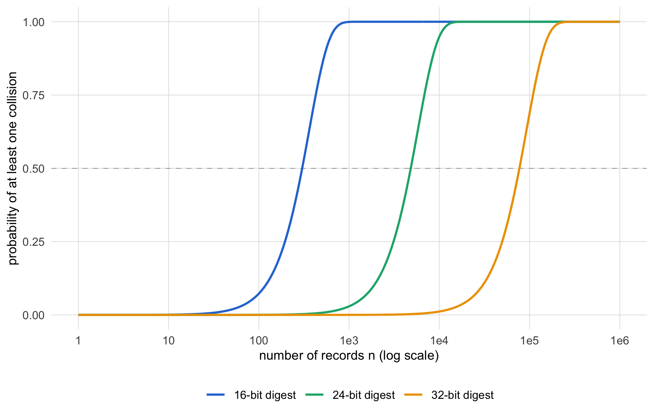
The three resistance notions are worth setting side by side, since the trial ledger leans on a different one for each of its guarantees (Table 3.1).
| Resistance property | Informal statement | Work factor | Ledger property it underwrites |
|---|---|---|---|
| Preimage | Given a digest, find any input that produces it | \(\sim 2^{n}\) | One-wayness: a published root leaks nothing about the records, and the leading-zeros search of proof-of-work |
| Second preimage | Given one record, find a different record with the same digest | \(\sim 2^{n}\) | No single committed record can be swapped for a chosen substitute |
| Collision | Find any two records that share a digest | \(\sim 2^{n/2}\) | Binding of the Merkle root: no record altered, added, or removed without changing the root |
3.4.2 The avalanche effect, measured
The avalanche property is the claim that flipping one input bit flips each of the 256 output bits independently with probability one half. We do not assume the claim; we validate it, in the sense a laboratory validates an assay against a known standard before trusting the readings it will later return on unknown samples. If true, the Hamming distance between the two digests (the number of differing bits out of 256) is a sum of 256 independent fair coins, hence \(\mathrm{Binomial}(256, 0.5)\), with mean 128 and standard deviation \(\sqrt{256 \cdot 0.25} = 8\). We test this directly: hash many random strings, flip their last character, rehash, and record the Hamming distance in bits.
hex_to_bits <- function(hex) {
  bytes <- strtoi(
    substring(hex, seq(1, nchar(hex), 2),
              seq(2, nchar(hex), 2)),
    base = 16L)
  bits <- vapply(bytes,
    function(b) as.integer(rev(intToBits(b)[1:8])),
    integer(8))
  as.vector(bits)
}

flip_last_char <- function(s) {
  n <- nchar(s)
  ch <- substr(s, n, n)
  repl <- if (ch == 'a') 'b' else 'a'
  paste0(substr(s, 1, n - 1), repl)
}

set.seed(1)
N <- 4000
strs <- paste0('msg-', sprintf('%05d', sample(1e6, N)))
ham <- vapply(strs, function(s) {
  b1 <- hex_to_bits(h(s))
  b2 <- hex_to_bits(h(flip_last_char(s)))
  sum(b1 != b2)
}, numeric(1))

c(mean = mean(ham), sd = sd(ham),
  binom_sd = sqrt(256 * 0.25))
#>       mean         sd   binom_sd
#> 128.045000   8.027645   8.000000
The empirical mean sits near 128 and the standard deviation near the \(\mathrm{Binomial}(256, 0.5)\) value of 8. The histogram, with the normal approximation to that binomial overlaid, makes the agreement visible.
library(ggplot2)
library(tibble)

ggplot(tibble(ham = ham), aes(ham)) +
  geom_histogram(aes(y = after_stat(density)),
                 bins = 30, fill = 'grey70',
                 colour = 'white') +
  stat_function(
    fun = function(x) dnorm(x, 128, sqrt(64)),
    linewidth = 0.8) +
  labs(x = 'Hamming distance (bits changed of 256)',
       y = 'density',
       title = 'Avalanche: one input bit flips ~half the output bits')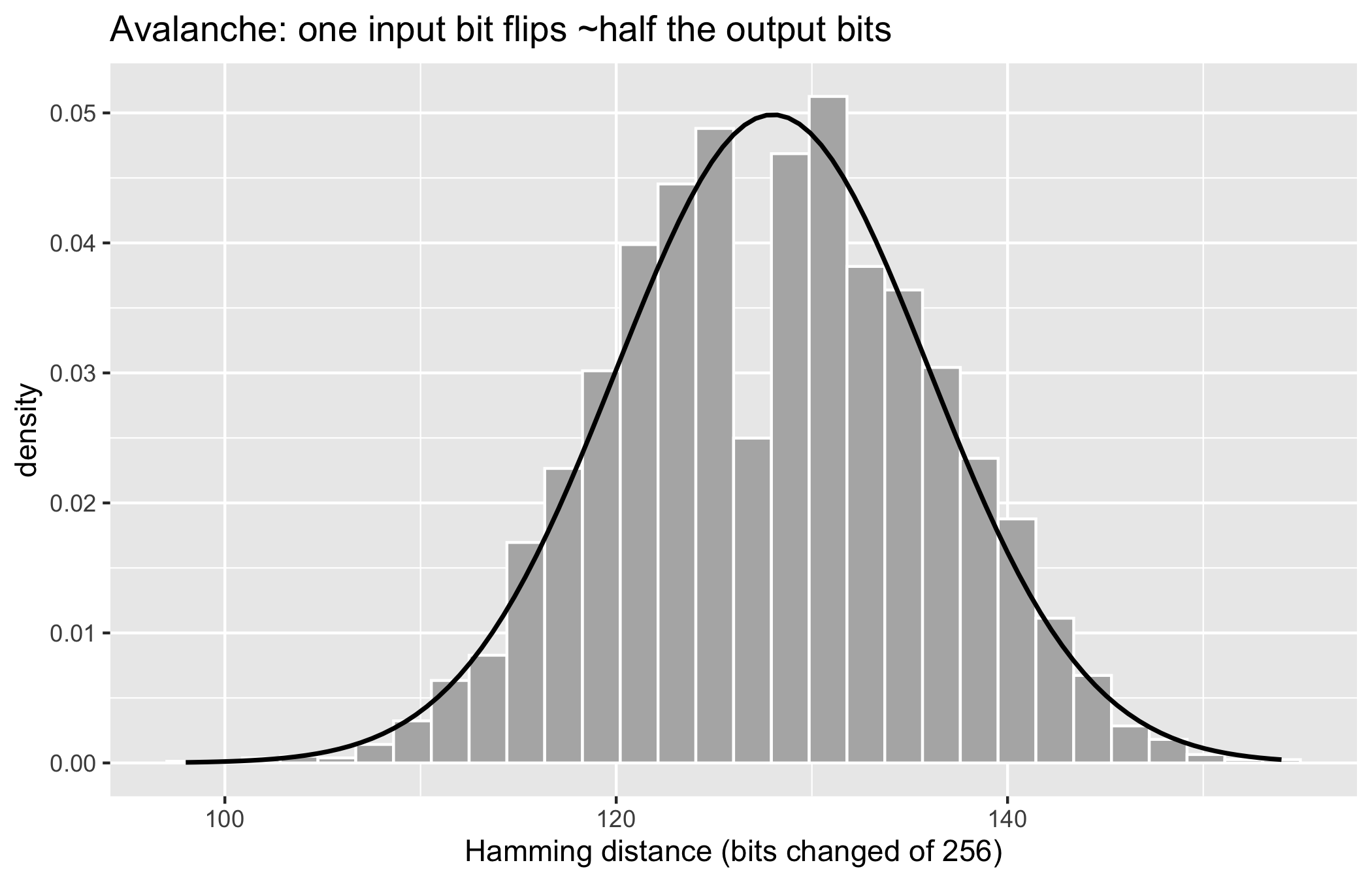
A single input change scrambles the output as if it were independently re-randomised. This is the avalanche property stated as a measurable fact. We should note the epistemic status carefully: the observed \(\mathrm{Binomial}(256, 0.5)\) shape is consistent with the random-oracle model, and it is what makes a one-character edit to a trial record betray itself. It is not a proof that SHA-256 has no exploitable structure, only that no structure shows up in this margin.
3.4.3 Uniformity of the output
Uniformity is the second observable consequence we validate, and we test it as we would test any claimed random-number generator before admitting it into a simulation. If digests are uniform on \(\{0,1\}^{256}\), then any fixed byte of the output is uniform on \(\{0,1,\dots,255\}\). We hash 50000 distinct inputs, tabulate the first output byte into its 256 cells, and apply a chi-square goodness-of-fit test against the uniform expectation.
set.seed(2)
M <- 50000
first_byte <- vapply(seq_len(M), function(i) {
  strtoi(substr(h(paste0('u-', i)), 1, 2),
         base = 16L)
}, numeric(1))

obs <- tabulate(first_byte + 1, nbins = 256)
chisq <- chisq.test(obs, p = rep(1 / 256, 256))
c(statistic = unname(chisq$statistic),
  df = unname(chisq$parameter),
  p_value = chisq$p.value)
#>   statistic          df     p_value
#> 221.4144000 255.0000000   0.9367624
The chi-square statistic sits near its degrees of freedom (255, the mean of a \(\chi^{2}_{255}\)) and the p-value is unremarkable. There is no evidence against uniformity of the first byte, consistent with a hash that behaves as a random oracle. The same caveat applies: this is a test of one marginal, and passing it is necessary but nowhere near sufficient for cryptographic security. A backdoored hash could pass every marginal test we can afford to run while failing catastrophically on a structured input the designer chose in advance.
ImportantThe sceptic’s reflex
Marketing copy calls encryption ‘military-grade’ and systems ‘unhackable’. Both phrases are tier-four narrative wearing the cadence of a protocol fact. ‘Military-grade’ names no property: AES-256 is excellent and freely available, and the adjective adds nothing measurable. ‘Unhackable’ is stronger and worse, because the security of every primitive in this chapter is conditional. Collision resistance holds only until someone finds a better-than-birthday attack, exactly as they did for MD5 and SHA-1. The correct claim is always quantitative and conditional: ‘finding a collision costs about \(2^{128}\) evaluations under current cryptanalysis’. When a vendor omits the number and the condition, demote the claim and ask for both.
3.5 Merkle trees
A Merkle tree, named for Ralph Merkle who introduced the hash-tree construction, turns a list of records into a single digest, the root, such that membership of any one record can be proven with a number of hashes logarithmic in the list length. Leaves are the hashes of the records; each internal node is the hash of its two children concatenated; the root is the hash at the top. Two facts make the structure useful, and both follow from the hash properties above. First, the root is a binding commitment: changing any record changes its leaf, which by collision resistance changes every ancestor up to the root. Second, proving that a record is in the tree requires revealing only the sibling hash at each level, \(\lceil \log_2 m \rceil\) hashes for \(m\) leaves, not the other \(m - 1\) records.
We implement the tree with the same h() from above. When a level has an odd number of nodes we duplicate the last one, the common convention that keeps the tree binary. This code is self-contained and additional to the verified companion blocks.
hash_pair <- function(a, b) h(paste0(a, b))

merkle_root <- function(leaves) {
  level <- vapply(leaves, h, character(1))
  while (length(level) > 1) {
    if (length(level) %% 2 == 1) {
      level <- c(level, level[length(level)])
    }
    idx <- seq(1, length(level), by = 2)
    level <- vapply(idx,
      function(i) hash_pair(level[i], level[i + 1]),
      character(1))
  }
  unname(level)
}

set.seed(101)
records <- paste0('trial-record-',
                  sprintf('%03d', 1:8))
root <- merkle_root(records)
root
#> [1] "08d101e1617dd700396b3d94548e46cff0771c028486560e06b5e140b8991050"
The eight synthetic records collapse to one 256-bit root. But how would a regulator check a single record without the whole database? This is what the inclusion proof provides. To prove that records[k] is committed, we walk from its leaf to the root, recording at each level the sibling hash and whether it sits to the left or the right. The verifier replays that walk from the leaf hash and checks that it reconstructs the published root.
merkle_proof <- function(leaves, index) {
  level <- vapply(leaves, h, character(1))
  proof <- list()
  i <- index
  while (length(level) > 1) {
    if (length(level) %% 2 == 1) {
      level <- c(level, level[length(level)])
    }
    # sibling is to the right of an odd (left) node,
    # to the left of an even (right) node
    if (i %% 2 == 1) {
      proof[[length(proof) + 1]] <-
        list(hash = unname(level[i + 1]),
             side = 'right')
    } else {
      proof[[length(proof) + 1]] <-
        list(hash = unname(level[i - 1]),
             side = 'left')
    }
    idx <- seq(1, length(level), by = 2)
    level <- vapply(idx,
      function(j) hash_pair(level[j], level[j + 1]),
      character(1))
    i <- (i + 1) %/% 2
  }
  proof
}

merkle_verify <- function(leaf, proof, root) {
  acc <- h(leaf)
  for (step in proof) {
    acc <- if (step$side == 'right')
             hash_pair(acc, step$hash)
           else hash_pair(step$hash, acc)
  }
  acc == root
}
We now demonstrate the three properties that make the structure worth its complexity: every genuine record verifies, a proof is logarithmic in size, and a forged record fails.
proof_3 <- merkle_proof(records, 3)

all_verify <- vapply(seq_along(records),
  function(k) merkle_verify(records[k],
    merkle_proof(records, k), root),
  logical(1))

c(all_leaves_verify = all(all_verify),
  proof_length = length(proof_3),
  log2_leaves = log2(length(records)),
  forged_leaf_verifies =
    merkle_verify('trial-record-forged',
                  proof_3, root))
#>    all_leaves_verify         proof_length          log2_leaves
#>                    1                    3                    3
#> forged_leaf_verifies
#>                    0
Every one of the eight records verifies against the root; the proof for a leaf is three hashes long, matching \(\log_2 8 = 3\); and a forged record presented with a genuine proof fails, because its leaf hash does not reconstruct the root. A light client holding only the 256-bit root can therefore confirm that a specific record belongs to a committed set of any size, receiving only \(\log_2 m\) hashes and none of the other records. That is the whole basis of simplified payment verification in Bitcoin, where a wallet verifies that a transaction is in a block using the block header’s Merkle root without downloading the block.
The proof path is easier seen than described. In Figure 3.3 we draw the eight-leaf tree of the code above and highlight the inclusion proof for the third leaf.
library(ggplot2)
library(tibble)

nodes <- tibble::tribble(
  ~x,  ~y, ~label,   ~role,
  1,   0, 'L1',     'other',
  2,   0, 'L2',     'other',
  3,   0, 'L3',     'target',
  4,   0, 'L4',     'sibling',
  5,   0, 'L5',     'other',
  6,   0, 'L6',     'other',
  7,   0, 'L7',     'other',
  8,   0, 'L8',     'other',
  1.5, 1, 'H(1:2)', 'sibling',
  3.5, 1, 'H(3:4)', 'path',
  5.5, 1, 'H(5:6)', 'other',
  7.5, 1, 'H(7:8)', 'other',
  2.5, 2, 'H(1:4)', 'path',
  6.5, 2, 'H(5:8)', 'sibling',
  4.5, 3, 'root',   'path')

edges <- tibble::tribble(
  ~x,  ~y, ~xend, ~yend, ~erole,
  1,   0, 1.5, 1, 'other',
  2,   0, 1.5, 1, 'other',
  3,   0, 3.5, 1, 'path',
  4,   0, 3.5, 1, 'sibling',
  5,   0, 5.5, 1, 'other',
  6,   0, 5.5, 1, 'other',
  7,   0, 7.5, 1, 'other',
  8,   0, 7.5, 1, 'other',
  1.5, 1, 2.5, 2, 'sibling',
  3.5, 1, 2.5, 2, 'path',
  5.5, 1, 6.5, 2, 'other',
  7.5, 1, 6.5, 2, 'other',
  2.5, 2, 4.5, 3, 'path',
  6.5, 2, 4.5, 3, 'sibling')

txt_col <- ifelse(nodes$role %in% c('target', 'path'),
                  'white', 'grey15')
nodes$role <- factor(nodes$role,
  levels = c('target', 'path', 'sibling', 'other'),
  labels = c('target leaf', 'recomputed path',
             'proof sibling', 'uninvolved'))

fill_named <- c('target leaf' = '#1d5a9e',
                'recomputed path' = '#2a78d6',
                'proof sibling' = '#eda100',
                'uninvolved' = '#9a9a92')
edge_cols <- c(path = '#2a78d6', sibling = '#eda100',
               other = 'grey80')

ggplot() +
  geom_segment(data = edges,
    aes(x = x, y = y, xend = xend, yend = yend,
        colour = erole),
    linewidth = 0.7, show.legend = FALSE) +
  scale_colour_manual(values = edge_cols) +
  geom_tile(data = nodes, aes(x = x, y = y, fill = role),
            width = 0.82, height = 0.55, colour = 'white') +
  geom_text(data = nodes, aes(x = x, y = y, label = label),
            colour = txt_col, size = 2.5) +
  scale_fill_manual(values = fill_named, name = NULL) +
  expand_limits(x = c(0.4, 8.6), y = c(-0.4, 3.5)) +
  theme_void(base_size = 11) +
  theme(legend.position = 'bottom')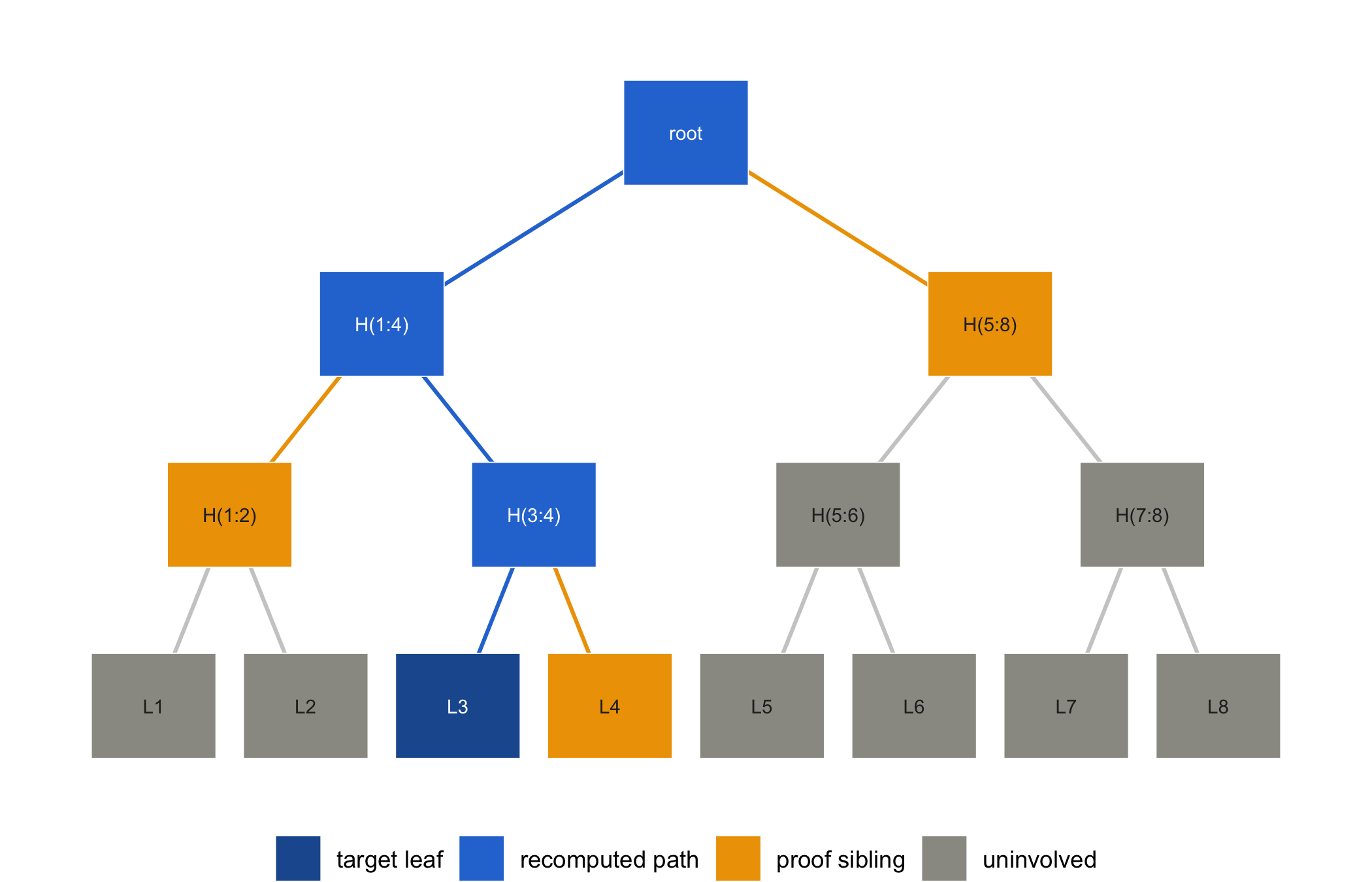
3.5.1 Public-health application: committing to a locked trial dataset
We return now to the problem with which the chapter opened, for here the cryptography is genuinely the right tool. At database lock the trial ledger fixes its dataset before unblinding and analysis. The recurring integrity question is whether any record was altered after lock, for example to remove an inconvenient adverse event or to adjust an outcome in a direction favourable to the sponsor. We build a Merkle tree over the hashes of the locked records and publish the root, whether in a journal, a registry, a timestamping service, or simply a widely-witnessed public post. The root is a 256-bit commitment to the entire dataset. Later, any party, and in particular the regulator of the opening scenario, may be handed a single record together with a logarithmic inclusion proof and verify that the record was in the locked set; and by collision resistance no record can be altered, added, or removed without changing the published root and thereby exposing the tampering. The records themselves never need to be disclosed in order to make the commitment, so patient confidentiality is preserved, since the published root reveals nothing about the data.
Figure 3.4 traces what the regulator sees when a single record is altered after lock.
library(ggplot2)
library(tibble)

tnodes <- tibble::tribble(
  ~x,  ~y, ~label,   ~role,
  1,   0, 'L1',     'other',
  2,   0, 'L2',     'other',
  3,   0, 'L3',     'other',
  4,   0, 'L4',     'other',
  5,   0, 'L5',     'other',
  6,   0, 'L6*',    'tampered',
  7,   0, 'L7',     'other',
  8,   0, 'L8',     'other',
  1.5, 1, 'H(1:2)', 'other',
  3.5, 1, 'H(3:4)', 'other',
  5.5, 1, 'H(5:6)', 'prop',
  7.5, 1, 'H(7:8)', 'other',
  2.5, 2, 'H(1:4)', 'other',
  6.5, 2, 'H(5:8)', 'prop',
  4.5, 3, 'root',   'prop')

tedges <- tibble::tribble(
  ~x,  ~y, ~xend, ~yend, ~erole,
  1,   0, 1.5, 1, 'other',
  2,   0, 1.5, 1, 'other',
  3,   0, 3.5, 1, 'other',
  4,   0, 3.5, 1, 'other',
  5,   0, 5.5, 1, 'other',
  6,   0, 5.5, 1, 'prop',
  7,   0, 7.5, 1, 'other',
  8,   0, 7.5, 1, 'other',
  1.5, 1, 2.5, 2, 'other',
  3.5, 1, 2.5, 2, 'other',
  5.5, 1, 6.5, 2, 'prop',
  7.5, 1, 6.5, 2, 'other',
  2.5, 2, 4.5, 3, 'other',
  6.5, 2, 4.5, 3, 'prop')

ttxt <- ifelse(tnodes$role %in% c('tampered', 'prop'),
               'white', 'grey15')
tnodes$role <- factor(tnodes$role,
  levels = c('tampered', 'prop', 'other'),
  labels = c('altered record', 'changed ancestry',
             'unchanged'))

tfill <- c('altered record' = '#e34948',
           'changed ancestry' = '#e34948',
           'unchanged' = '#9a9a92')
tedge <- c(prop = '#e34948', other = 'grey80')

ggplot() +
  geom_segment(data = tedges,
    aes(x = x, y = y, xend = xend, yend = yend,
        colour = erole),
    linewidth = 0.7, show.legend = FALSE) +
  scale_colour_manual(values = tedge) +
  geom_tile(data = tnodes, aes(x = x, y = y, fill = role),
            width = 0.82, height = 0.55, colour = 'white') +
  geom_text(data = tnodes, aes(x = x, y = y, label = label),
            colour = ttxt, size = 2.5) +
  annotate('text', x = 4.5, y = 3.6,
           label = 'root no longer matches the regulator copy',
           colour = '#e34948', size = 2.8) +
  scale_fill_manual(values = tfill, name = NULL) +
  expand_limits(x = c(0.4, 8.6), y = c(-0.4, 3.9)) +
  theme_void(base_size = 11) +
  theme(legend.position = 'bottom')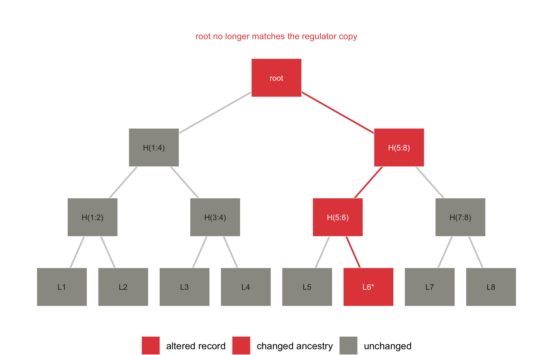
WarningThis needs no blockchain
The mechanism above is a hash tree and a published root. It requires no consensus protocol, no tokens, no mining, and no chain. A single trustworthy publication of the root at lock is sufficient, because the security rests entirely on collision resistance, not on distributed agreement. A blockchain would add value only if no party could be trusted even to publish the root honestly and promptly, which is rarely the situation in a regulated trial with an established registry. This is the falsifiability discipline of Chapter 1 in action: the useful primitive here is the Merkle commitment, and attaching ‘blockchain’ to it is tier-four narrative unless a specific trust failure is named that only consensus can repair. The timestamping lineage that predates blockchains (Haber & Stornetta, 1991) made exactly this point: tamper-evident chronology is a hashing problem, and was solved as one.
3.6 Digital signatures over elliptic curves
Hashing makes the trial ledger tamper-evident; signatures make its entries attributable. The Merkle commitment settles whether a record was altered, but it says nothing about who entered it. In the trial ledger we also wish to know which site coordinator recorded a given eCRF entry, and to have that attribution be checkable by a party, such as the regulator, who trusts none of the coordinators in advance. The public-key idea (Diffie & Hellman, 1976; Rivest et al., 1978) supplies exactly this: a signer holds a private scalar and publishes a corresponding public key, such that anyone can verify a signature but only the holder of the private key can produce one. A coordinator who signs each entry with a site-held private key makes authorship of that entry cryptographically checkable, and forging an attribution is as hard as the discrete-logarithm problem we come to below. Blockchains realise this over elliptic-curve groups, and the group that matters for Bitcoin and much of Ethereum is secp256k1: the points \((x, y)\) satisfying \(y^{2} = x^{3} + 7\) over the prime field \(\mathbb{F}_{p}\) for a specific 256-bit prime \(p\), together with a point at infinity as the identity. These points form a cyclic group of prime order, generated by a fixed base point \(G\).
The group law is geometric: to add two points, draw the line through them, find its third intersection with the curve, and reflect across the \(x\)-axis. A private key is a scalar \(d\); the public key is the point \(Q = dG\), meaning \(G\) added to itself \(d\) times (computed efficiently by double-and-add, not \(d\) literal additions). Recovering \(d\) from \(Q\) and \(G\) is the elliptic-curve discrete logarithm problem, believed to require about \(2^{128}\) operations for secp256k1. That asymmetry, easy to multiply the base point by a scalar, infeasible to invert, is the wall between a public key and its private scalar.
To make the group concrete we verify the one axiom that is not obvious from the geometry, associativity, on a small curve \(y^{2} = x^{3} + ax + b\) over \(\mathbb{F}_{97}\). The arithmetic is identical in kind to secp256k1; only the field is small enough to enumerate.
mod_inv <- function(a, p) {
  a <- a %% p
  for (x in 1:(p - 1)) if ((a * x) %% p == 1) return(x)
  stop('no inverse')
}

# Curve: y^2 = x^3 + a x + b over F_p,
# with the point at infinity as NA.
ec_add <- function(P, Q, a, p) {
  if (all(is.na(P))) return(Q)
  if (all(is.na(Q))) return(P)
  if (P[1] == Q[1] && (P[2] + Q[2]) %% p == 0)
    return(c(NA, NA))
  if (all(P == Q)) {
    m <- ((3 * P[1]^2 + a) * mod_inv(2 * P[2], p)) %% p
  } else {
    m <- ((Q[2] - P[2]) *
          mod_inv((Q[1] - P[1]) %% p, p)) %% p
  }
  xr <- (m^2 - P[1] - Q[1]) %% p
  yr <- (m * (P[1] - xr) - P[2]) %% p
  c(xr %% p, yr %% p)
}

p <- 97; a <- 2; b <- 3
pts <- do.call(rbind, Filter(Negate(is.null),
  lapply(0:(p - 1), function(x) {
    y2 <- (x^3 + a * x + b) %% p
    ys <- which(((0:(p - 1))^2 %% p) == y2) - 1
    if (length(ys)) cbind(x, ys) else NULL
  })))

P <- pts[3, ]; Q <- pts[5, ]; R <- pts[9, ]
lhs <- ec_add(ec_add(P, Q, a, p), R, a, p)
rhs <- ec_add(P, ec_add(Q, R, a, p), a, p)
list(P = P, Q = Q, R = R,
     associative = isTRUE(all.equal(lhs, rhs)),
     result = lhs)
#> $P
#>  x ys
#>  1 43
#>
#> $Q
#>  x ys
#>  3  6
#>
#> $R
#>  x ys
#> 10 21
#>
#> $associative
#> [1] TRUE
#>
#> $result
#> ys ys
#> 80 87
Associativity holds: \((P + Q) + R\) equals \(P + (Q + R)\). With associativity, an identity, and inverses (the reflection of a point), the points form an abelian group, and scalar multiplication \(dG\) is well-defined. Inverting it, the discrete-log problem, is the hardness the signature scheme rests on.
3.6.1 ECDSA, Schnorr, and aggregation
Two signature schemes run on this group. ECDSA is the scheme Bitcoin launched with: to sign a message digest \(m\) with private key \(d\), the signer draws a per-signature nonce \(k\), computes a point \(kG\), and produces a pair \((r, s)\) where the algebra binds \(m\), \(d\), \(r\), and \(k\). ECDSA works, but its security is fragile in one notorious way: reusing or leaking the nonce \(k\) across two signatures leaks the private key algebraically, and a biased \(k\) leaks it statistically. The nonce is a place where a subtle random-number-generator flaw becomes a total key compromise, which is a lesson in why the uniformity tests earlier in this chapter are not academic.
Schnorr signatures, named for Claus Schnorr who proposed them (Schnorr, 1991), achieve the same authentication with a cleaner algebraic structure. Because the Schnorr verification equation is linear in the key and the nonce, signatures and keys can be aggregated: several signers can produce a single signature valid for the sum of their public keys, and a batch of signatures can be verified together faster than one at a time. Aggregation is attractive for a blockchain because signatures dominate transaction size and verification cost; combining \(n\) signatures into one shrinks both. This linearity is why Bitcoin’s Taproot upgrade adopted Schnorr.
BLS signatures, named for Boneh, Lynn and Shacham (Boneh et al., 2001), push aggregation further using a pairing on a suitable curve. A BLS signature is a single group element, and, crucially, signatures from many signers on the same message aggregate into one short signature verifiable against the aggregate public key. This is the property that makes BLS the signature scheme of choice for proof-of-stake consensus in Chapter 10, where thousands of validators attest to each block and the ability to compress thousands of signatures into one is what keeps the protocol tractable.
3.6.2 A note on quantum threats
We should not close the discussion of signatures without asking how durable their hardness is, for a question that once seemed academic has become a genuine design consideration. What would a large-scale quantum computer do to the primitives of this chapter? The answer divides sharply, and the division is the practical point. Shor’s algorithm solves the discrete-logarithm and integer- factorisation problems in polynomial time, and these are precisely the problems on which ECDSA and RSA rest. A sufficiently large quantum computer would therefore recover a private key from its public key and forge signatures at will, which is to say that the public-key signatures of this chapter would fail completely rather than merely weaken. Hash functions fare far better. Grover’s algorithm speeds an unstructured search only quadratically, so inverting an \(n\)-bit hash falls from about \(2^{n}\) to about \(2^{n/2}\) work; a hash loses roughly a square-root factor of its security and no more, which for SHA-256 still leaves a comfortable \(2^{128}\). The analysis of quantum attacks on Bitcoin by Aggarwal and colleagues (Aggarwal et al., 2018) works these asymmetries through in detail and reaches the same qualitative conclusion: signatures are the exposed surface, and hashes are relatively robust.
For a health ledger the implication is not hypothetical, and it turns on the longevity of the record. A trial ledger is a long-lived object: a signature made today to attribute an eCRF entry may need to remain unforgeable for decades, through the archival life of the trial and any later re-analysis or litigation. This is the ‘harvest now, forge later’ horizon, in which an adversary records today’s public keys and signatures and waits for the cryptographic era to turn, at which point yesterday’s unforgeable attributions become forgeable. The horizon is genuine for any ledger meant to outlive the current generation of public-key cryptography, and it argues, on the one hand, for preferring hash-based commitments wherever a hash will do the work, since these are the resilient primitive, and, on the other, for designing the signature layer to be replaceable, so that a migration to a post-quantum scheme can be carried out without discarding the ledger. We do not attempt to recommend a specific post-quantum signature here; the field is still settling, and the prudent posture, in our view, is to keep the option open rather than to commit early.
3.7 Commitments and zero-knowledge
The Merkle root is one instance of a commitment: a short value that binds a party to hidden data (binding), while revealing nothing about it until opened (hiding). The same idea generalises. A commitment scheme lets a party publish a commitment now and reveal the committed value later, with the scheme guaranteeing the value cannot be changed in between. The binding property rests on collision resistance, exactly as the Merkle root does, and the hiding property on the one-wayness of the hash, so a commitment asks of the reader nothing that the present chapter has not already supplied.
A commitment fixes a value, but it does not, by itself, let one demonstrate anything about that value while it remains hidden. That further step, proving a property of committed data without opening it, is the province of the zero-knowledge proof, to which we now turn.
3.8 Zero-knowledge proofs
We begin with a claim that sounds paradoxical and is not. Can one party convince another that a statement is true while conveying nothing whatever beyond its truth, not even the reason it is true? The affirmative answer, formalised by Goldwasser, Micali and Rackoff (Goldwasser et al., 1989), whose study of the knowledge complexity of interactive proof systems founded the subject, is among the deeper results of modern cryptography, and it rests on three properties that a reader trained in statistics will find unusually congenial. Consider a prover, who claims to hold a witness to some statement, and a verifier, who will accept or reject after an exchange of messages. An interactive proof system is required to satisfy three conditions.
- Completeness. If the statement is true and the prover is honest, the verifier accepts with overwhelming probability. An honest prover in possession of the witness is essentially never turned away.
- Soundness. If the statement is false, then no prover, however devious, can make the verifier accept except with some small probability, the soundness error. This error is not a defect to be apologised for; it is the very quantity the construction controls, and repetition drives it toward zero.
- Zero-knowledge. The verifier learns nothing from the exchange beyond the truth of the statement, in the precise sense that whatever the verifier sees could have been simulated, without the prover at all, from the statement alone.
The property that repays statistical attention is soundness, and it is worth dwelling on why. A soundness error of \(\varepsilon\) means that a cheating prover, one who does not hold the witness, slips a false statement past the verifier with probability at most \(\varepsilon\) on a single run. But how small must \(\varepsilon\) be? Here the analogy to hypothesis testing is exact rather than decorative. The verifier is running a test whose null hypothesis is ‘the prover does not know the witness’, and the soundness error is precisely the type-one error rate, the probability of accepting a false claim. A single round of a protocol whose challenge is one bit has soundness error one half, which no statistician would accept as a test. There are then two routes to a small error, and they are interchangeable. One may repeat the protocol: because the rounds are independent, \(t\) repetitions drive the soundness error to \(2^{-t}\), the geometric decay that Figure 3.5 traces against the conventional 0.05 level. Or one may widen the challenge within a single round, so that a prover who can answer only one of the \(\lvert C \rvert\) possible challenges for a given commitment succeeds with probability at most \(1 / \lvert C \rvert\). The Schnorr protocol below takes the second route, drawing its challenge from the whole scalar field, and so attains a negligible soundness error in one round with no repetition at all; the repetition picture belongs to its small-challenge cousins. One chooses whichever route the setting favours to meet the tolerance demanded.
library(ggplot2)
library(tibble)

PAL <- c('#2a78d6', '#1baf7a', '#eda100', '#008300',
         '#4a3aa7', '#e34948', '#e87ba4', '#eb6834')

book_theme <- theme_minimal(base_size = 11) +
  theme(
    panel.grid.minor = element_blank(),
    panel.grid.major = element_line(
      linewidth = 0.25, colour = 'grey88'),
    axis.title = element_text(size = 10),
    legend.position = 'bottom')

rounds <- 0:12
sound <- tibble::tibble(t = rounds, err = (1 / 2)^rounds)

ggplot(sound, aes(t, err)) +
  geom_hline(yintercept = 0.05, linewidth = 0.25,
             colour = 'grey60', linetype = 2) +
  geom_line(linewidth = 0.8, colour = PAL[1]) +
  geom_point(size = 1.6, colour = PAL[1]) +
  annotate('text', x = 9, y = 0.075,
           label = 'conventional 0.05 level',
           colour = 'grey40', size = 2.8) +
  scale_y_log10(breaks = 10^(0:-4),
                labels = c('1', '0.1', '0.01',
                           '0.001', '0.0001')) +
  scale_x_continuous(breaks = seq(0, 12, 2)) +
  labs(x = 'number of independent rounds t',
       y = 'soundness error (log scale)') +
  book_theme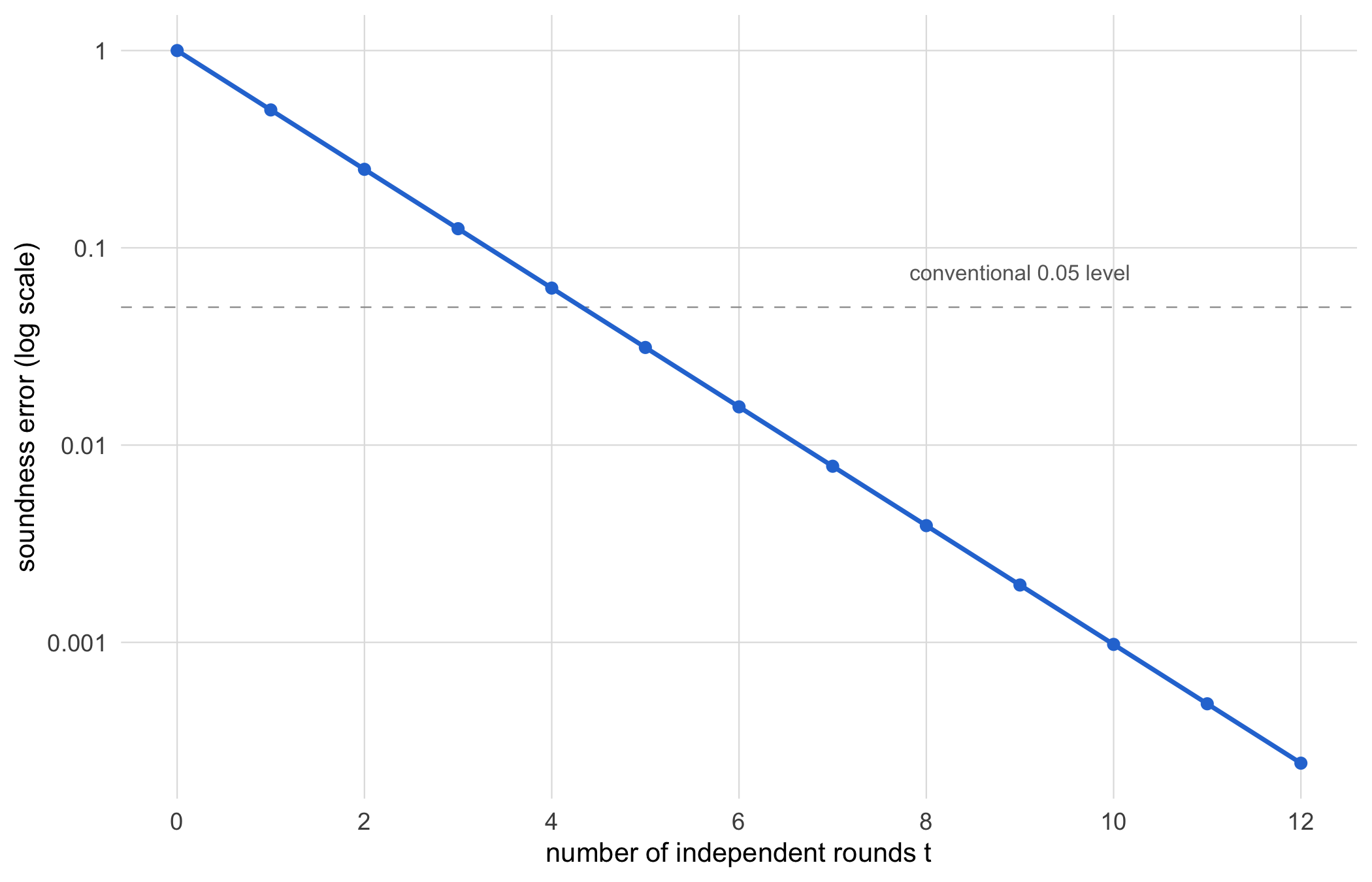
The abstraction becomes concrete in the oldest and cleanest example, the identification protocol of Schnorr (Schnorr, 1991). Recall the elliptic-curve group of the preceding section, with base point \(G\) of prime order and the discrete-logarithm problem, recovering \(d\) from \(Q = dG\), believed hard. A prover wishes to convince a verifier that she knows the private scalar \(d\) behind a public key \(Q = dG\), without revealing \(d\). The exchange has the three-move shape that names this family of protocols, the sigma-protocol, after the shape of its message flow.
- Commitment. The prover draws a fresh random scalar \(r\), computes the point \(R = rG\), and sends \(R\). The scalar \(r\) is a secret nonce, and its role is exactly that of a commitment: it binds the prover to a value she cannot afterward change.
- Challenge. The verifier draws a random scalar \(c\) and returns it. This is the public coin, chosen after the commitment is fixed.
- Response. The prover sends \(s = r + c\,d\), computed with the secret scalars, and the verifier accepts if \(sG\) equals \(R + cQ\).
The algebra closes because \(sG = (r + c\,d)G = rG + c(dG) = R + cQ\), so an honest prover always passes, which is completeness. Soundness is the interesting direction: a prover who does not know \(d\) cannot in general answer a challenge she could not predict, and one can show that a prover able to answer two different challenges for the same commitment \(R\) would thereby reveal \(d\) outright, which is the knowledge-extraction argument that gives the soundness its teeth. The protocol is zero-knowledge because the triple \((R, c, s)\) can be simulated without \(d\) at all: choose \(s\) and \(c\) at random and set \(R = sG - cQ\), and the resulting transcript is distributed exactly as a genuine run, carrying no information about the secret. That last observation is the whole content of the zero-knowledge property in miniature.
One inconvenience remains. The protocol as described is interactive, in that the verifier must be present to issue the challenge \(c\). But what if the prover wishes to leave behind a proof that anyone can check later, with no live verifier at all? The device that removes the verifier is the Fiat-Shamir heuristic, and its intuition is simple. The challenge is meant to be unpredictable to the prover before she commits, and a cryptographic hash, which the earlier part of this chapter established behaves as a random oracle, supplies exactly such unpredictability. We replace the verifier’s coin with \(c = H(R, \text{statement})\), the hash of the commitment together with the statement being proved. The prover cannot steer the output of the hash, and so cannot choose \(R\) to suit a favourable \(c\); the interactive protocol collapses to a single non-interactive proof, the pair \((R, s)\), that any party can verify by recomputing the challenge. This is, incidentally, how the interactive identification scheme becomes the Schnorr signature met earlier, and it is one more reason the random-oracle tests of this chapter are load-bearing rather than ornamental.
The Schnorr proof is small and quick, but its statement is fixed and simple, namely knowledge of one discrete logarithm. The ambition of the last decade has been to prove, just as compactly, that an arbitrary computation was carried out correctly, that a whole batch of transactions is valid, or that a committed record satisfies an elaborate predicate. The proofs that achieve this go by the name of succinct non-interactive arguments of knowledge, or SNARKs. What does ‘succinct’ buy? It is the property that the proof is far smaller than the computation it attests to and can be checked in far less time than re-executing that computation would take, so that a verifier who would need hours to redo the work can instead check a proof of a few hundred bytes in milliseconds. Ben-Sasson, Chiesa, Tromer and Virza (Ben-Sasson, Chiesa, Tromer, et al., 2014) gave a construction for a general von Neumann computer architecture, bringing arbitrary programs within reach; Groth (Groth, 2016) produced the compact pairing-based scheme, with proofs of constant size, that is now widely deployed; and Ben-Sasson and colleagues (Ben-Sasson et al., 2018) later introduced transparent STARKs, which dispense with the trusted setup that pairing-based SNARKs require and rest their security on hashes alone, at the cost of somewhat larger proofs. The application that turned these ideas from theory into consequence was Zerocash (Ben-Sasson, Chiesa, Garman, et al., 2014), which used succinct proofs to build a payment system in which a transaction proves its own validity, that its inputs and outputs balance and the spender is authorised, while revealing neither sender, receiver, nor amount, and so turned zero-knowledge into private payments.
We should be candid about the boundary of our competence here. The internal machinery of these constructions, the arithmetic circuits, the polynomial commitments, the elliptic-curve pairings, is a substantial body of cryptographic engineering that lies well beyond the scope of this book. We cite these systems as an interface and not as an implementation: what matters for our purposes is the guarantee they expose, a short proof that a stated computation was performed correctly, and not the mechanism by which they attain it.
Why should a book concerned with public-health data attend to any of this? Because zero-knowledge is the natural language for privacy-preserving health analytics, and the connection is not merely metaphorical. To illustrate, consider a multi-site trial with an eligibility protocol under which a prospective participant must fall within an age band and carry a laboratory value in a specified range. A site can, in principle, prove to the coordinating centre that a given individual satisfies these criteria, that the age lies in one interval and the lab value in another, without transmitting the date of birth or the laboratory result itself. The statement ‘this record satisfies the predicate’ is established; the record stays home. Broadened, this is the same aspiration as secure multiparty computation and federated analysis, in which a statistic, a regression coefficient or a pooled prevalence, is computed jointly across institutions while each retains custody of its raw data and surrenders none of it.
The analogy must be drawn with care, for it is easily overstated. A zero-knowledge proof establishes the truth of a statement about data that has already been committed; it does not, on its own, compute a joint statistic across parties. Proving that each site’s record satisfies a predicate is a different operation from combining those records into a pooled estimate, and the latter is the province of secure multiparty computation proper, of which zero-knowledge proofs are a component rather than a synonym. We flag the distinction because conflating the two is a common route to overstating what a privacy-preserving pipeline actually delivers. The constructions themselves we take no further here, and the reader who wishes to pursue them is referred to the primary sources named above.
Before the worked example we gather the four primitives of the chapter into one view, each with the guarantee it provides and, as important, the guarantee it does not (Table 3.2).
| Primitive | Guarantee | Role in the trial ledger | What it cannot do |
|---|---|---|---|
| Hash | Deterministic one-way fingerprint | Detects any change to a record | Attribute authorship, or reveal what changed beyond the digest |
| Digital signature | Authenticity and non-repudiation | Attributes each eCRF entry to a site coordinator | Prove integrity of anything beyond what was signed, or establish time |
| Merkle tree | Logarithmic membership proof over a binding root | Lets an auditor verify one record against the root without the dataset | Say who entered a record, or when |
| Commitment | Binding and hiding | Publishes a value now to be revealed later, fixed in between | Prove a property of the hidden value, which needs zero-knowledge |
3.9 Worked example
To illustrate, consider the trial ledger at its lock date, with the pieces now assembled into one end-to-end analysis of the problem with which we began. We commit to the locked dataset, prove one record’s membership to an auditor, and confirm that any tampering is caught by the published root. This is the trial-ledger application of the previous section, run as code on a SYNTHETIC locked dataset standing in for the real trial records.
set.seed(303)

# SYNTHETIC locked trial dataset: one row per
# subject, serialised to a canonical string.
locked <- data.frame(
  subject = sprintf('S%04d', 1:16),
  arm = sample(c('A', 'B'), 16, replace = TRUE),
  outcome = rbinom(16, 1, 0.3),
  stringsAsFactors = FALSE
)
record_strings <- with(locked,
  paste(subject, arm, outcome, sep = '|'))

published_root <- merkle_root(record_strings)

# An auditor is handed subject 7's record plus a
# proof, and verifies membership against the
# published root alone.
k <- 7
audit_ok <- merkle_verify(
  record_strings[k],
  merkle_proof(record_strings, k),
  published_root)

# Someone alters subject 12's outcome after lock.
tampered <- record_strings
tampered[12] <- paste0(tampered[12], '-edited')

c(auditor_confirms_membership = audit_ok,
  proof_hashes = length(merkle_proof(record_strings, k)),
  tamper_changes_root =
    merkle_root(tampered) != published_root)
#> auditor_confirms_membership                proof_hashes
#>                           1                           4
#>         tamper_changes_root
#>                           1
The auditor confirms subject 7’s record with a four-hash proof (the tree over 16 leaves has depth four) and never sees the other fifteen records. The post-lock edit to subject 12 changes the root, so anyone holding the originally published root detects that the dataset is no longer the one committed to. The guarantee is exactly as strong as collision resistance, which the birthday analysis priced at about \(2^{128}\) work, and no stronger. It is also, as the warning above insisted, achieved with no blockchain: a hash tree and one honest publication.
3.10 Collaborating with an LLM
Language models are fluent about cryptography and confidently wrong at its edges, which is precisely where security lives. They are of use in accelerating routine work, provided the parts that matter are verified against a primary source.
Prompt. ‘Write an R function to compute a Merkle root and an inclusion proof using the digest package.’
Watch for: the odd-node convention (duplicate the last node, or promote it unchanged?), off-by-one errors in sibling indexing, and whether the proof records left/right order at all. A verifier that ignores order will accept proofs for the wrong position.
Verification: the structural checks in this chapter’s demo (every leaf verifies, a forged leaf fails, tampering changes the root) are the minimum. These are correctness checks on the implementation, not a security proof of the scheme.
Prompt. ‘Explain why collision resistance is weaker than preimage resistance for a 256-bit hash.’
Watch for: confident but reversed statements. Models sometimes assert collisions cost \(2^{256}\), missing the birthday factor entirely, or garble which property protects which use case.
Verification: the reader should re-derive the birthday bound independently (\(m \approx 2^{n/2}\)) and check the model’s numbers against it. The truncated-hash simulation in this chapter is a fast empirical cross-check.
Prompt. ‘Is it safe to reuse the same nonce across two ECDSA signatures?’
Watch for: any answer that does not immediately say this leaks the private key. Nonce reuse is a catastrophic, well-documented failure, and a model that hedges is a warning about the model.
Verification: consult the scheme’s specification, not the model, for anything a key depends on. Treat LLM cryptography as a tier-two claim requiring a primary source.
3.11 Exercises
Birthday bound by simulation. Extend the
first_collision()function to truncation widths of 8, 12, 16, and 20 bits. For each, estimate the mean first-collision count over several hundred replications and plot it against \(\sqrt{\pi N/2}\) on log axes. Confirm the slope corresponds to the \(2^{n/2}\) law and report the fitted exponent.-
Leading-zeros work. Verify empirically that the expected number of SHA-256 evaluations to find a digest with \(k\) leading zero bits is \(2^{k}\). Estimate the mean trial count for \(k = 8, 12, 16\) and compare to \(2^{k}\). Explain how this experiment is the kernel of proof-of-work in
Avalanche at the byte level. The chapter tested avalanche in bits. Repeat the analysis counting differing bytes out of 32 instead of bits out of 256, derive the distribution differing bytes should follow under the random oracle, and test the fit. (Hint: a byte differs with probability \(1 - 2^{-8}\).)
Merkle proof forgery. Attempt to construct a valid inclusion proof for a record not in the tree, without finding a hash collision. Argue from the
merkle_verify()logic why this reduces to finding a preimage or collision, and state which resistance property each forgery strategy would have to defeat.Second-preimage on a truncated hash. Using truncation to make it feasible, empirically estimate the work to find a second input hashing to the same truncated digest as a fixed target, and confirm it scales as \(2^{b}\) rather than \(2^{b/2}\). Explain why this differs from the collision experiment in exercise 1.
Group order. For the toy curve \(y^{2} = x^{3} + 2x + 3\) over \(\mathbb{F}_{97}\), enumerate all points (the chapter’s
ptsmatrix, plus the point at infinity) and count them. Verify that the count equals the group order, and check Lagrange’s theorem by confirming that the order of a chosen point divides it.
3.12 Further reading
The Merkle tree originates with Merkle (1988), which introduces the hash tree as a way to sign many messages from one public value; read it for the construction in its original framing. The timestamping papers of Haber & Stornetta (1991) are the direct ancestors of the tamper-evident-log idea and make explicit that chronology and integrity are hashing problems, a useful corrective to blockchain-first accounts. For public-key cryptography, Diffie & Hellman (1976) is the conceptual origin and Rivest et al. (1978) the first concrete realisation; both are short and worth reading as primary sources.
On signatures, Schnorr (1991) introduces the scheme whose linearity underlies modern aggregation, and Boneh et al. (2001) introduces the short pairing-based signatures that make proof-of-stake consensus tractable at Chapter 10 scale. The zero-knowledge framework is Goldwasser et al. (1989), foundational for the privacy constructions later chapters build on. For the primitives in blockchain context, Narayanan et al. (2016) (chapters 1 and 4) gives the rigorous treatment this chapter matches to a statistical audience, and Antonopoulos (2017) gives the concrete Bitcoin realisations of hashing, Merkle trees, and ECDSA. The proof-of-work use of the leading-zeros bound traces to Back (2002), which 1 develops in full.
3.13 In conclusion
In conclusion, three points are to be emphasised. First, the security of every mechanism in this chapter is quantitative and conditional, resolved into a specific cost under current cryptanalysis (preimage resistance at about \(2^{n}\), collision resistance at about \(2^{n/2}\) by the birthday bound), and never the flat ‘unbreakable’ of marketing copy; an analyst who conflates the two resistance properties will overstate by the square root of the security exponent. Second, the statistical tests we ran on the hash validate the random-oracle model as one validates an assay, establishing that the output is consistent with the model at the margins we were able to examine while establishing nothing about structure we did not test, and the distinction between failing to reject uniformity and proving security is the whole of the discipline. Third, for the trial ledger the right primitive is the Merkle commitment to the locked dataset, which needs no blockchain, and the statistician’s contribution lies as much in declining to reach for consensus machinery that a single honest publication renders unnecessary as in deploying the cryptography where a genuine trust failure warrants it.