11 On-Chain Data Analysis and Tokenomics
Bitcoin has the unintuitive property that while the ownership of money is implicitly anonymous, its flow is globally visible.
Meiklejohn et al., A Fistful of Bitcoins (2013)
11.1 Learning objectives
By the end of this chapter the reader should be able to:
- Frame the analysis of a public ledger as an observational study, and name the selection, confounding, and measurement threats that attach to it.
- Treat address clustering as an entity- resolution problem, apply the common-input- ownership heuristic, and state why pseudonymity is not anonymity.
- Quantify wealth concentration with a Lorenz curve and a Gini coefficient, and explain why concentration is security-relevant under proof-of-stake.
- Fit and honestly test a block-interval model, and locate where the exponential assumption is expected to fail on real data.
- Read a token’s economics through market capitalisation versus fully diluted valuation, build an unlock schedule, and give an operational test for ‘Ponzinomics’.
- Keep a scored forecasting log, compute a Brier score, and read a calibration curve, closing the falsifiability programme of Chapter 1.
11.2 Orientation
We open, and shall in due course close the book, with a single auditing question. Given an append-only data store, whether a public blockchain or a health registry that no custodian may quietly overwrite, what can we honestly infer from it, and how do we keep our own claims honest while we do so? The question is older than blockchains. It is the question an epidemiologist asks of any record assembled without a controlled design, and this closing chapter is, in the end, an epidemiology of a ledger.
The preceding chapters treated blockchains as mechanisms: a consensus protocol to be analysed, a cryptographic primitive to be measured, a market to be modelled. This chapter treats a blockchain as something else, a dataset. Every confirmed transaction on a public chain is a permanent, world-readable record, and the aggregate is one of the largest openly available behavioural datasets in existence. For a statistician this is the payoff of everything that came before: the guarantees established in Chapter 2 and Chapter 3 are exactly what make the data trustworthy enough to analyse.
It will help to fix a concrete public-health instance of the same auditing problem, and we shall carry it through the chapter. Consider several hospitals that agree to share one append-only record of a multi-centre clinical trial. Each enrolment, each randomisation, and each outcome event is written to a ledger that no single institution owns and none may silently revise, and a regulator audits the record after the fact. We shall refer to this arrangement throughout as the trial ledger. A vaccine cold-chain provenance system, in which each custody transfer of a refrigerated lot is committed to a shared log, is a second instance we shall reach for where it illuminates a point. Both are append-only stores that a distrustful party must audit after the fact, which is precisely the situation the on-chain analyst faces.
The central discipline of the chapter is to remember what kind of dataset it is. On-chain data is observational, not experimental. Nobody randomised addresses into treatment arms. The population of participants is self-selected, the measured quantities are proxies for the latent quantities of interest, and the generating process is adversarial, for some of the entities in the data are actively trying to be misclassified. Every caution a biostatistician brings to an electronic health record or an insurance claims database applies here, and a few more besides.
The reader already owns the tools, under other names. Wealth concentration is a Lorenz curve and a Gini coefficient (Kondor et al. (2014), an empirical study of the concentration of Bitcoin holdings), the very instruments of health-inequity measurement. Block arrivals are a renewal process (a sequence of independent waiting times between successive events) whose fit can be tested (Chapter 5). De-anonymisation is entity resolution, the record-linkage problem of registry deduplication (Meiklejohn et al. (2013), the study of Meiklejohn and colleagues that clustered the Bitcoin address graph into economic actors). Token release is a deterministic schedule whose future supply is a piece of cohort bookkeeping, computable today. The work of the chapter is to apply these familiar instruments to an unfamiliar substrate, and to report the results with the honesty that observational data demands. We take up each in turn: the observational-study framing in the next section, then clustering, concentration, the block-interval model, tokenomics, and finally the forecasting log with which the book closes.
Several terms recur through the chapter, and we gather the least familiar of them here so that the reader need not hold them as mysteries while the argument proceeds.
- On-chain data. The permanent, world-readable record of confirmed transactions on a public blockchain, read here as an observational dataset rather than as a designed experiment.
- Address clustering (entity resolution). The grouping of many pseudonymous addresses into the single economic actor that controls them. The workhorse rule is the common-input-ownership heuristic: when one transaction spends several inputs together, all those input addresses are presumed to belong to one owner, since the spender had to sign for each. It is the record-linkage problem of a patient registry applied to a ledger.
- Pseudonymity versus anonymity. Pseudonymity hides only the map from addresses to identities while leaving every transaction permanently public; anonymity would hide the activity itself. A chain is pseudonymous, and pseudonymity degrades under analysis.
- Mixer. A service that pools funds from many users and redistributes them, deliberately breaking the input-output linkage on which clustering depends.
- Market capitalisation versus fully diluted valuation (FDV). Market capitalisation is the circulating supply times price; FDV is the total eventual supply times price. The gap between them is the value of the supply not yet released.
- Total value locked (TVL). The token value deposited in a protocol, denominated in the very tokens whose prices it aggregates, and therefore not a direct measure of adoption or of safety.
- Vesting and unlock schedule. The deterministic timetable, fixed in a token’s contract, by which allocated but locked tokens (to a team, to early investors) become circulating, each unlock adding to the effective supply.
- Ponzinomics. A token structure in which the returns paid to existing participants are funded from the capital of new entrants rather than from any revenue exogenous to the token.
Because each instrument arrives under a name the reader already owns, we set the correspondence out in one place before we begin. Table 11.1 pairs each on-chain tool with its public-health twin and the caveat both inherit, so that the rest of the chapter can be read as a single method applied to two substrates.
| On-chain tool | Public-health twin | Shared caveat |
|---|---|---|
| Address clustering (common-input-ownership) | Record linkage and capture-recapture | A heuristic classifier; false and missed matches must be reported, not hidden |
| Gini and Lorenz concentration | Health-inequity measurement | The unit of analysis (address versus entity) sets the number before any estimator does |
| Block-interval fit | Survival and arrival-time diagnostics | A pooled fit can pass while the stress regimes one cares about fail |
| Unlock schedule | Cohort follow-up accrual | Deterministic today, but only as far as the vesting contract is honoured |
| Brier calibration | Epidemic-forecast scoring | A low score is not calibration; the log must be kept prospectively |
11.3 The statistician’s contribution
Before turning to the instruments, we should name three judgements that are the analyst’s own, for no tool performs them for us.
Reading a chain as an observational study, not a ledger of facts. A transaction graph is a sample, not a census of economic behaviour, and it is a biased sample: the entities that transact on-chain differ systematically from those that do not, custodial addresses aggregate many users behind one pseudonym, and wash trading, the practice of trading with oneself to fabricate the appearance of activity, manufactures volume. Naming the estimand, and the gap between it and what the chain actually measures, is prior to any number.
Operationalising a narrative into a test. The field runs on unfalsifiable claims: ‘decentralised’, ‘sound money’, ‘sustainable yield’. The statistician’s contribution is to convert each into a measurable quantity with a rejection region. ‘Decentralised’ becomes a Gini coefficient on stake. ‘Sustainable yield’ becomes a question about whether returns are paid from exogenous cash flow or from new entrants. Once a claim has been given a test it can be shown false, which is the entire purpose of formulating it.
Scoring one’s own forecasts. Scepticism that is never recorded and never graded is merely a posture. The calibration log introduced in Chapter 1 and closed here holds the analyst’s own predictions to the same standard demanded of the promoters: a probability, an outcome, and a Brier score. A well-calibrated critic is of more value than a loud one.
The second judgement is the engine of the whole chapter, so we make its machinery explicit. Table 11.2 sorts a claim into one of the four falsifiability tiers of Chapter 1 and names, for each tier, the test that would settle it. The same ladder governs a crypto slogan and a public-health assertion, and the analyst’s task is to keep pushing a claim down the ladder until it names an outcome that could arrive and prove it wrong.
| Tier | Crypto claim | Health claim | Test that settles it |
|---|---|---|---|
| 1 Protocol fact | The contract releases 30% of supply at month 12 | The registry recorded 400 enrolments | Read it off the ledger or registry; deterministic |
| 2 Empirical | Active addresses rose 40% this quarter | Coverage reached 80% in the district | Measure it from records, with the error stated |
| 3 Model-dependent | This staking yield is sustainable | This vaccine prevents 60% of cases | Fix the model and estimator; report assumptions and fit |
| 4 Narrative | The chain is decentralised | The programme is a success | Not falsifiable until forced down to a tier-2 measurement |
PAL <- c('#2a78d6', '#1baf7a', '#eda100', '#008300',
         '#4a3aa7', '#e34948', '#e87ba4', '#eb6834')

book_theme <- ggplot2::theme_minimal(base_size = 11) +
  ggplot2::theme(
    panel.grid.minor = ggplot2::element_blank(),
    panel.grid.major = ggplot2::element_line(
      linewidth = 0.25, colour = 'grey88'),
    axis.title = ggplot2::element_text(size = 10),
    legend.position = 'bottom'
  )
11.4 A chain is an observational dataset
We consider the estimand before the estimator. Suppose we want the distribution of wealth among the economic participants of a chain. What the ledger gives us is the distribution of balances across addresses. These are not the same object, and the map between them is exactly the source of every serious error in on-chain analysis. The statistician who has audited a disease registry will recognise the difficulty at once, for it is the difficulty of any observational study: the quantity we can measure is not, in general, the quantity we should like to have measured.
An address is a public key, not a person. One person may control thousands of addresses, and one address, an exchange’s hot wallet, that is, the online account it uses for day-to-day settlement, may hold the pooled balances of millions of people. The unit of observation the chain hands us is therefore not the unit of analysis we want. This is a measurement problem in the precise sense of the term, for the observed variable is a noisy, biased, and non-injective function of the latent variable.
To name the hazards is to recite the epidemiologic catechism unchanged. Three classical threats organise the caution.
- Selection. The set of addresses that ever transact is self-selected and unrepresentative of any wider population. Inferences about ‘people’ from a chain are inferences about a peculiar, wealthy, technically sophisticated, and partly automated subpopulation.
- Confounding. Apparent relationships in the transaction graph are routinely driven by unobserved common causes: a single market maker, a single exploit, a single exchange’s internal rebalancing. Correlation of address activity is weak evidence of a relationship between distinct economic actors.
- Measurement. Balances, volumes, and active- address counts are proxies. Volume can be fabricated by wash trading at near-zero cost. Active-address counts are inflated by dust, that is, economically negligible amounts scattered across many addresses, and by wallet software that splits change across new addresses. The proxy and the target diverge, and the divergence is not random.
The methodological posture that follows is the one a biostatistician already holds toward registry data, and it transfers to the trial ledger without amendment. The data is real and valuable, the access is unusually complete, and precisely for that reason the temptation to treat a proxy as its target is unusually strong. On the one hand the completeness of an append-only record is a genuine analytic gift; on the other, completeness is not representativeness, and a census of addresses is still not a census of people.
11.5 Address clustering and de-anonymisation
Bitcoin is pseudonymous, not anonymous, and the distinction is the entire content of Meiklejohn et al. (2013). Every transaction is public forever, and what is hidden is only the map from addresses to identities. Recovering part of that map is a statistical problem the reader will recognise immediately, for it is entity resolution, the record-linkage task that deduplicates a patient registry or links records across health databases that share no common key. The epidemiologist who has estimated the size of a hidden population by capture-recapture, matching individuals across incomplete lists, has already practised the core move: we accumulate partial identifying evidence until distinct records resolve into one entity.
The workhorse is the common-input-ownership heuristic. When a transaction spends several inputs at once, the spender had to sign for all of them, so under normal wallet behaviour all those input addresses are controlled by one entity. Each multi-input transaction is therefore an assertion that its input addresses belong to the same cluster. Accumulating these assertions is a union-find (disjoint-set) computation: addresses are nodes, co-spending is an edge, and the connected components are candidate entities.
Figure 11.1 draws the move in the small. Six pseudonymous addresses carry co-spending edges that merge them into two entities, while one exchange address, though a single node, fronts many users behind one pseudonym and so is the measurement error the section warns against, drawn in red.
ellipse <- function(cx, cy, rx, ry, grp, n = 80) {
  t <- seq(0, 2 * pi, length.out = n)
  tibble(x = cx + rx * cos(t), y = cy + ry * sin(t), grp = grp)
}

# SYNTHETIC layout: six addresses, three co-spending
# edges, one exchange fronting several users.
nodes <- tibble(
  id = c('a1', 'a2', 'a3', 'a4', 'a5', 'exchange'),
  x  = c(1.1, 2.1, 1.7, 4.9, 5.9, 8.4),
  y  = c(3.7, 3.9, 2.6, 3.8, 2.9, 3.2),
  kind = c('addr', 'addr', 'addr', 'addr', 'addr', 'exchange')
)
edges <- tibble(
  x    = c(1.1, 1.7, 4.9),
  y    = c(3.7, 2.6, 3.8),
  xend = c(2.1, 2.1, 5.9),
  yend = c(3.9, 3.9, 2.9)
)
hulls <- bind_rows(
  ellipse(1.6, 3.4, 1.0, 1.0, 'entity 1'),
  ellipse(5.4, 3.35, 0.85, 0.9, 'entity 2')
)
users <- tibble(x = c(9.0, 9.25, 9.0), y = c(3.9, 3.2, 2.5))

ggplot() +
  geom_path(data = hulls, aes(x, y, group = grp, colour = grp),
            linewidth = 0.7) +
  geom_segment(data = edges, aes(x, y, xend = xend, yend = yend),
               colour = '#33356b', linewidth = 0.6) +
  geom_point(data = filter(nodes, kind == 'addr'), aes(x, y),
             colour = '#33356b', size = 5) +
  geom_point(data = users, aes(x, y), colour = '#9a9a92', size = 2.4) +
  geom_segment(data = users, aes(x = 8.4, y = 3.2, xend = x, yend = y),
               colour = '#9a9a92', linewidth = 0.3) +
  geom_point(data = filter(nodes, kind == 'exchange'), aes(x, y),
             colour = '#e34948', size = 6) +
  geom_text(data = filter(nodes, kind == 'addr'), aes(x, y, label = id),
            colour = 'white', size = 3) +
  annotate('text', x = 1.6, y = 4.65, label = 'entity 1',
           colour = PAL[1], size = 3.3) +
  annotate('text', x = 5.4, y = 4.55, label = 'entity 2',
           colour = PAL[2], size = 3.3) +
  annotate('text', x = 8.4, y = 1.7,
           label = 'exchange: many users,\none pseudonym',
           colour = '#e34948', size = 3.1) +
  scale_colour_manual(values = c('entity 1' = PAL[1],
                                 'entity 2' = PAL[2])) +
  expand_limits(y = c(1.3, 4.9)) +
  coord_equal(clip = 'off') +
  guides(colour = 'none') +
  theme_void()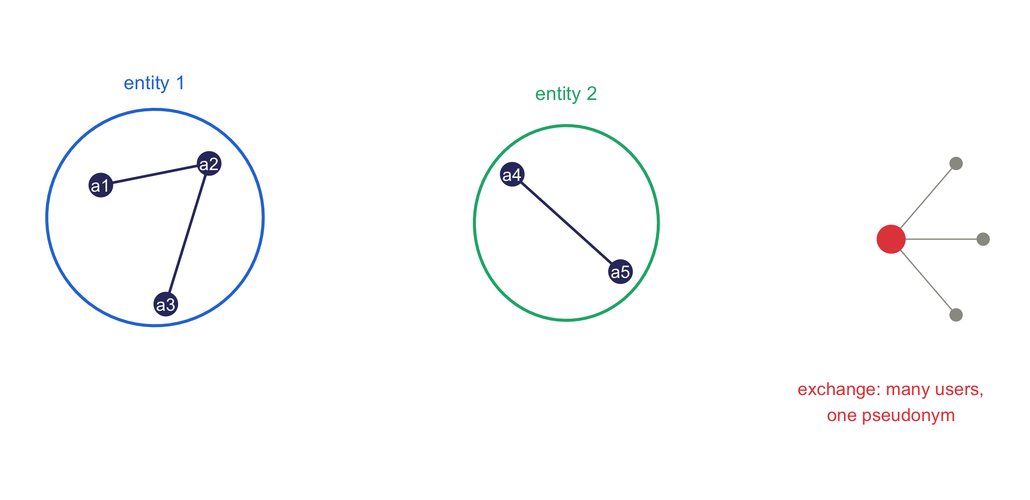
set.seed(21)
# SYNTHETIC: 800 transactions co-spending among
# 300 pseudonymous addresses. Real wallets reuse
# addresses, so co-spending links accumulate.
n_addr <- 300
n_tx <- 800
tx_inputs <- replicate(
  n_tx,
  sample(n_addr, size = sample(1:3, 1)),
  simplify = FALSE
)

parent <- seq_len(n_addr)
uf_find <- function(i) {
  while (parent[i] != i) i <- parent[i]
  i
}
uf_union <- function(a, b) {
  ra <- uf_find(a)
  rb <- uf_find(b)
  if (ra != rb) parent[rb] <<- ra
}

for (ins in tx_inputs) {
  if (length(ins) > 1L) {
    for (k in 2:length(ins)) uf_union(ins[1], ins[k])
  }
}

roots <- vapply(seq_len(n_addr), uf_find, integer(1))
c(addresses = n_addr,
  entities = length(unique(roots)),
  largest_cluster = max(tabulate(roots)))
#>       addresses        entities largest_cluster
#>             300               5             296
We see the 300 pseudonymous addresses collapse into far fewer entities, and a single super-cluster emerges, the familiar giant component of a random graph past its percolation threshold. This is SYNTHETIC data, but the qualitative result is the one Meiklejohn et al. (2013) obtained on the real Bitcoin graph: a modest set of heuristics, applied at scale, reduces a pseudonymous ledger to a tractable number of economic actors, many of which can then be tagged by their interactions with known services. The same collapse is what a registry statistician calls deduplication, and it is neither more nor less than that here.
The heuristic is a classifier, and like any classifier it makes errors. CoinJoin transactions, which several independent users construct jointly, deliberately violate common-input-ownership by having many independent signers co-spend, injecting false-positive links, and wallets that avoid address reuse suppress true-positive links. We should therefore report the heuristic’s assumptions and its failure modes rather than present the clustering as ground truth, exactly as one would report the false-match and missed-match rates of a probabilistic record-linkage model in a registry study.
‘The blockchain is anonymous’ is a tier-four narrative delivered in the cadence of a tier-one protocol fact. The protocol fact is the opposite: the ledger is permanently and globally public, and only the identity map is hidden. Pseudonymity degrades under analysis, and it degrades retroactively, because the data never expires. A transaction that is unlinkable today may be de-anonymised by a heuristic or a subpoena years from now. Any claim of on-chain privacy must name the specific technique that provides it (a mixer, a zero-knowledge scheme) and the adversary it is proven against, or it is marketing.
11.5.1 Public-health relevance
The same machinery that de-anonymises a payment ledger de-anonymises a health-data store published under pseudonyms, and here the trial ledger demands a word of caution. If the consortium commits an append-only log of patient events under per-patient pseudonyms, the linkage structure of the events, that is, which pseudonyms co-occur in which records, is itself identifying, exactly as co-spending is identifying on Bitcoin. The lesson transfers without modification: pseudonymised health data on a public ledger is a re-identification dataset waiting for a heuristic, and the permanence of the ledger means the risk only grows rather than decays. We state the warning plainly, for it is the privacy corollary of the whole section: pseudonymity is not anonymity, on a chain or in a registry. This is a decisive argument against writing patient-level records, even pseudonymised ones, to any public chain, and it is why the trial ledger of our running example commits only integrity hashes and access-controlled pointers, never the clinical payload itself.
11.5.2 The de-anonymisation arms race
The heuristics of the previous section are not the end of the story but a move in a continuing game. Each advance in clustering has provoked a countermeasure, and each countermeasure has provoked a counter-countermeasure, so that the practical privacy of a chain is best read not as a settled fact but as the current state of an arms race. Meiklejohn and colleagues showed that a modest set of heuristics could collapse a pseudonymous ledger into a tractable set of economic actors (Meiklejohn et al. (2013)), and the response was a family of privacy technologies engineered precisely to defeat that collapse.
Two of these responses mark out the design space. The first is the mixing service, which pools funds from many users and redistributes them, so that the input-output linkage on which common-input-ownership depends is deliberately broken: the several inputs of a joint transaction are no longer one entity, and the heuristic that read co-spending as co-ownership now records a false positive. The second is the privacy-by-design chain, which builds concealment into the protocol rather than bolting it on afterward, and here two contrasting constructions merit mention. Monero hides the true spender among a set of decoys using ring signatures (a scheme in which a signature is valid for any member of a group, so that the true signer cannot be singled out), whereas Zerocash, the construction of Ben-Sasson and colleagues that underlies the Zcash chain, conceals the transaction graph altogether behind zero-knowledge shielded transactions (Ben-Sasson et al. (2014)). The latter is the zero-knowledge machinery of Chapter 3 put to work: a shielded transfer proves that a valid spend occurred without revealing the sender, the receiver, or the amount.
But does privacy-by-design settle the question in the user’s favour? It does not, and here the honest finding is two-sided. On the one hand the clustering literature shows that pseudonymity leaks, for the heuristics recover far more structure than the naive user expects. On the other hand the privacy tools are themselves fallible. Moser and colleagues, in a traceability study of Monero, traced a substantial fraction of its inputs by exploiting weaknesses in the early decoy sampling (Möser et al. (2018)), which is to say that a concealment scheme is only as strong as its implementation and its parameters. Neither anonymity nor de-anonymisation is therefore absolute. The practical privacy of a given user is an empirical and moving quantity, revised with each new heuristic and each new countermeasure, and it is emphatically not a theorem. Table 11.3 sets the exchange of moves out in one place, with the health-data analogue of each.
| Clustering move | On-chain countermeasure | Health-data analogue |
|---|---|---|
| Common-input-ownership heuristic | A mixing service pools and redistributes funds, breaking the input-output linkage | Aggregation or k-anonymity over quasi-identifiers |
| Tagging clusters by known services | A fresh address per payment; privacy-by-design chains | Pseudonym rotation and cell suppression |
| Decoy and ring-signature analysis | Larger, better-sampled decoy sets (Monero) | Adding noise or synthetic records to a release |
| Following the transaction graph | Zero-knowledge shielded transactions (Zcash) | Formal privacy guarantees inside a governed enclave |
The reader who works with health data has met this arms race before, under another name. The re-identification literature established long ago that a small number of quasi-identifiers, a postcode, a date of birth, a sex, can single out an individual in a release published as de-identified. A biostatistician who has absorbed that result already understands the mixer problem without further instruction, for it is the same problem: pseudonymity is not anonymity, on a chain or in a registry, and the privacy of a released dataset is a property to be tested empirically against a motivated adversary, not asserted by the custodian who released it. The mixing service and the k-anonymity transform, which coarsens a release until every record is indistinguishable from at least k-1 others, are two answers to one question, namely how much identifying structure survives an adversary who is actively trying to recover it.
Where does the parallel end? It ends at permanence and reach. A quasi-identifier attack on a health release is mounted by whoever holds the release, within a data enclave whose access can in principle be controlled, revoked, and audited. An on-chain pseudonym, by contrast, is permanent and world-readable: the data never expires and the adversary set is everyone, indefinitely. A linkage that is infeasible today may become feasible tomorrow with a better heuristic, or with an auxiliary dataset that does not yet exist, and the ledger will still be there to receive it. The arms race is thus the same game, but played on a chain for considerably higher stakes, which is one further reason the trial ledger of our running example commits only integrity proofs and keeps every identifying datum in a store that can still be locked.
11.6 Wealth concentration: Lorenz and Gini
The most-cited empirical fact about on-chain wealth is its concentration, and the instrument is one every reader has already used to measure health inequity, whether across incomes, insurance coverage, or the reach of a vaccination campaign. The Lorenz curve plots the cumulative share of total wealth held by the poorest fraction \(p\) of addresses, and the Gini coefficient is twice the area between that curve and the line of perfect equality. For a population \(x_1 \le \dots \le x_n\) the Gini has the convenient closed form
\[ G = \frac{2 \sum_{i=1}^{n} i\, x_i} {n \sum_{i=1}^{n} x_i} - \frac{n+1}{n}, \]
which we implement directly rather than reaching for a package. We test it on a heavy-tailed balance distribution, the SYNTHETIC stand-in for the log-normal-to-power-law shape that on-chain balances reliably exhibit.
gini_coef <- function(x) {
  x <- sort(x)
  n <- length(x)
  (2 * sum(seq_len(n) * x) / (n * sum(x))) - (n + 1) / n
}

set.seed(14)
# SYNTHETIC: heavy-tailed balances (log-normal),
# typical of on-chain balance distributions.
balances <- rlnorm(10000, meanlog = 0, sdlog = 2)
c(gini = gini_coef(balances),
  top1pct_share = sum(sort(balances, decreasing = TRUE)[1:100]) /
    sum(balances))
#>          gini top1pct_share
#>     0.8479588     0.3949864
The Gini sits high and the top one percent of addresses hold a large share of the total, the qualitative signature Kondor et al. (2014) documented for Bitcoin’s real balance distribution.
To illustrate that the instrument is indifferent to its substrate, consider the same coefficient applied not to token balances but to vaccine coverage. Suppose an immunisation programme reports the number of fully immunised children in each of eight districts as 950, 910, 880, 840, 300, 120, 60 and 20. A national average would look tolerable, yet the coefficient exposes the two districts carrying almost no coverage.
# SYNTHETIC: fully immunised children in eight
# districts. The same gini_coef, now measuring
# health inequity rather than token wealth.
coverage <- c(950, 910, 880, 840, 300, 120, 60, 20)
c(gini = gini_coef(coverage),
  bottom2_share = sum(sort(coverage)[1:2]) / sum(coverage))
#>          gini bottom2_share
#>    0.41605392    0.01960784
The Gini here carries exactly the meaning it carries on balances, namely that nearer zero is nearer parity and nearer one is nearer to a few districts holding all the coverage. The instrument does not change when the substrate changes from stake to sera; only the estimand does. A student who has quantified inequity in vaccination has therefore already met every idea in this section. To see the concentration rather than summarise it, we draw the Lorenz curve. The few lines below sort the balances, form the cumulative wealth share against the cumulative population share, and compare the result to the diagonal of perfect equality.
lorenz_curve <- function(x) {
  x <- sort(x)
  n <- length(x)
  tibble(
    pop_share = c(0, seq_len(n) / n),
    wealth_share = c(0, cumsum(x) / sum(x))
  )
}

lc <- lorenz_curve(balances)

ggplot(lc, aes(pop_share, wealth_share)) +
  geom_abline(linetype = 2) +
  geom_line(linewidth = 0.8) +
  coord_equal() +
  labs(x = 'cumulative share of addresses',
       y = 'cumulative share of wealth',
       title = 'Lorenz curve of on-chain balances (SYNTHETIC)')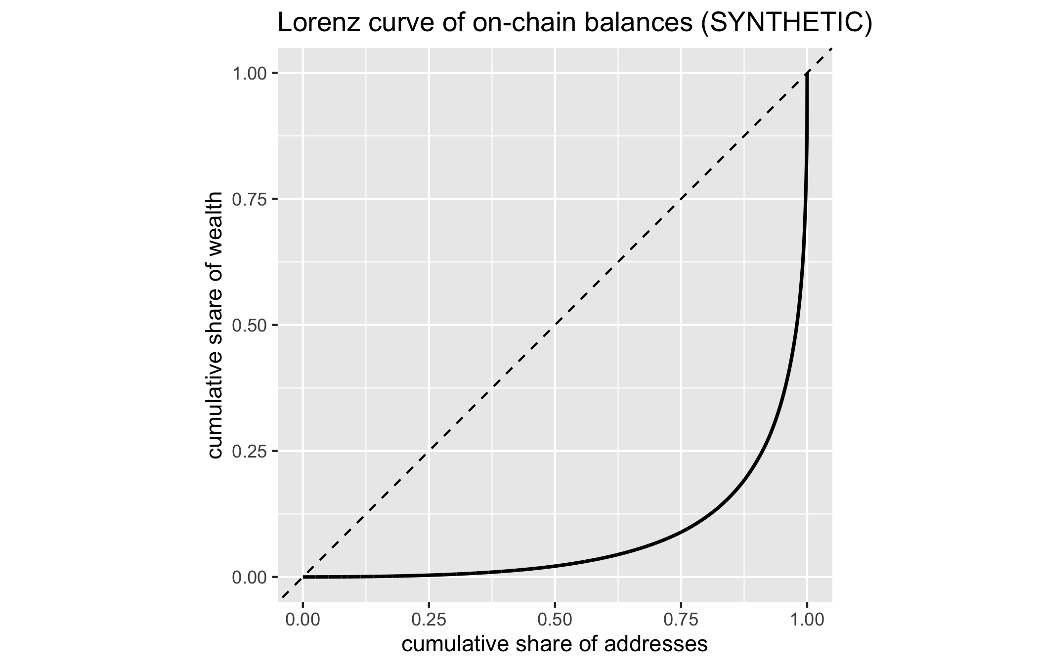
The curve bows far below the diagonal: the poorest ninety percent of addresses hold a negligible fraction of the wealth, while the top sliver holds almost all of it. For a proof-of-work chain this is a distributional curiosity. For a proof-of-stake chain it is a security parameter. Sybil resistance, the property that an actor cannot gain disproportionate influence merely by creating many identities, under proof-of-stake (Chapter 10, Douceur (2002)) presumes that influence is proportional to stake and that stake is not trivially concentrated in a few hands. A high stake Gini means a small number of entities approach the thresholds that matter for liveness and finality, and the clustering of Meiklejohn et al. (2013) can make the effective concentration worse than the address-level Gini suggests, because addresses that look independent may resolve to one staking entity. Concentration measurement is thus not sociological commentary; it is an input to the safety analysis.
11.7 Block-interval modelling on data
Chapter 5 derived the block interval as an exponential random variable, the memoryless waiting time of a Poisson process whose rate the difficulty controller holds near a set-point. Here we treat a series of intervals as data and ask whether the model survives contact with it. The workflow is the one any analyst applies to a distributional hypothesis: we estimate the rate, run a goodness-of-fit test, and inspect a QQ plot. It is the same workflow an epidemiologist brings to the spacing of events in a surveillance stream, and on the trial ledger it is the workflow that would test whether enrolments arrive as a steady Poisson process or in suspicious bursts.
set.seed(13)
# SYNTHETIC: intervals from Exp(mean 600s), the very
# model under test. Replace with a real CoinMetrics
# CSV to make this a genuine test of a real chain.
intervals <- rexp(2016, rate = 1 / 600)

fit_rate <- 1 / mean(intervals)
ks <- ks.test(intervals, 'pexp', rate = fit_rate)
c(mean_interval = mean(intervals), fitted_rate = fit_rate,
  ks_p_value = ks$p.value)
#> mean_interval   fitted_rate    ks_p_value
#>  6.041721e+02  1.655158e-03  5.352700e-01

ggplot(tibble(x = sort(intervals),
              theo = qexp(ppoints(length(intervals)), fit_rate)),
       aes(theo, x)) +
  geom_point(size = 0.6) + geom_abline(linetype = 2) +
  labs(x = 'exponential quantiles', y = 'observed intervals',
       title = 'Block intervals vs fitted exponential (SYNTHETIC)')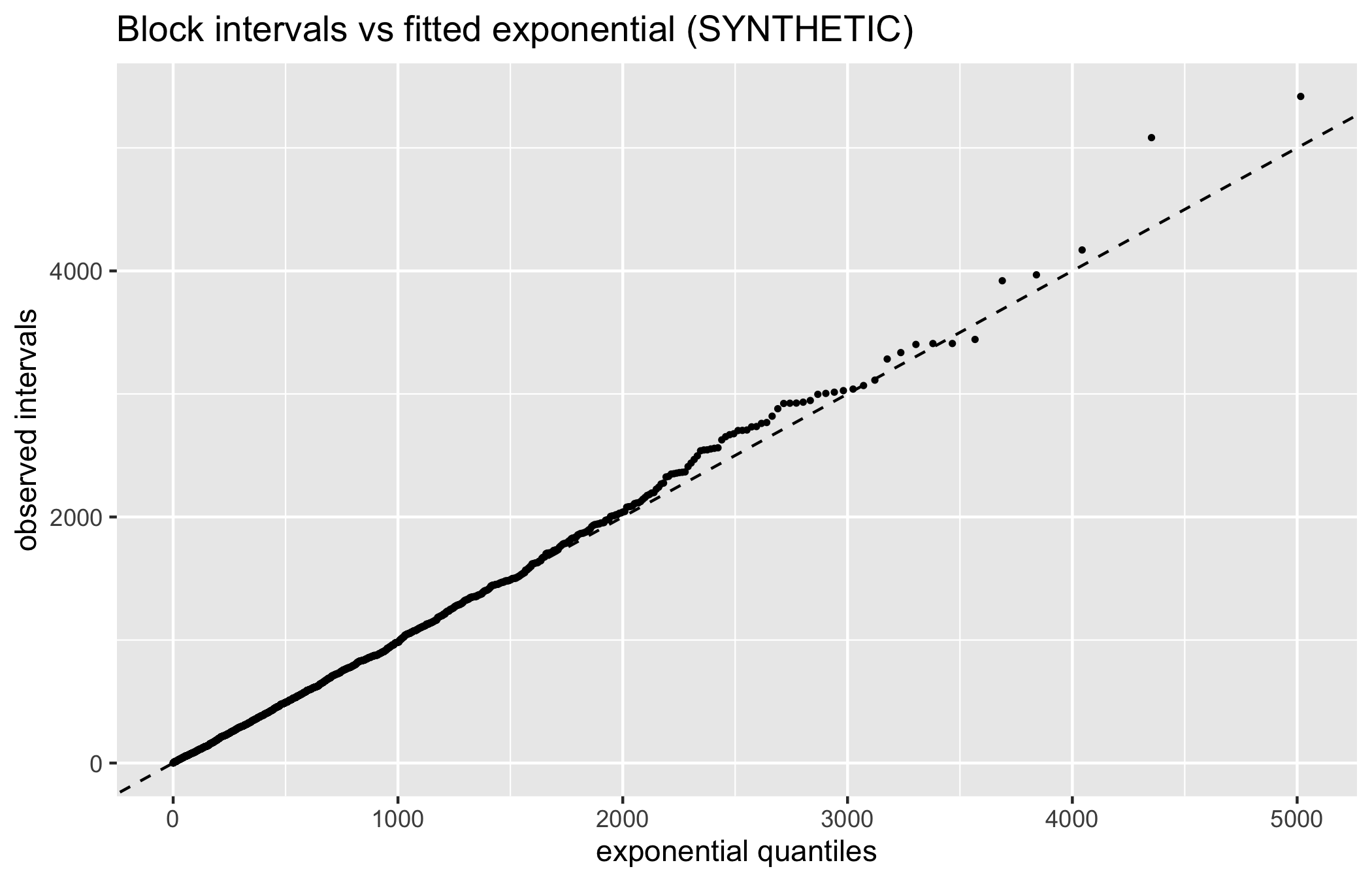
The QQ points lie on the diagonal and the Kolmogorov-Smirnov test does not reject, because we drew from the model. That is the point of the SYNTHETIC exercise: it establishes what a passing result looks like, so that a failure on real data is legible. On a real chain the interesting science is precisely where the exponential frays. Around a difficulty retarget, the periodic adjustment that resets the mining difficulty toward the target block time, the rate parameter is stale, so intervals cluster short or long until the controller catches up. During a hash-rate shock, the exogenous migration of miners, the interval distribution develops a heavy right tail that the single-rate exponential cannot represent. A memoryless model also cannot express the serial dependence that these episodes induce. Reporting where the fit breaks, and resisting the urge to declare victory because the bulk of the distribution looks exponential, is the deliverable. A model that fits the easy 95 percent and fails exactly during the stress events one cares about is worse than useless if its failure is not disclosed.
11.8 Tokenomics and the sceptic’s rubric
Tokenomics is the study of a token’s supply schedule and the claims made about its value. Almost all of it reduces to arithmetic that the promotional literature is structured to obscure. The first and most consequential distinction is between market capitalisation and fully diluted valuation.
Market capitalisation is the circulating supply times price. Fully diluted valuation (FDV) is the total eventual supply times price. When a large fraction of the supply has not yet been released, these two numbers diverge by an order of magnitude, and the released supply is the numerator that keeps the price up while the unreleased supply is a schedule of future sell pressure. A token can look cheap on market cap and be enormously expensive on FDV, and the gap is not an opinion; it is on the vesting contract.
Three headline valuations circulate, and each misleads in its own way, so we set their definitions against what inflates them and when a number may be trusted. Table 11.4 is the reference we return to whenever a dashboard quotes one figure and suppresses the other two.
| Metric | Definition | What inflates it | When to trust it |
|---|---|---|---|
| Market cap | Circulating supply times price | A low float that suppresses the circulating count | Only when paired with FDV and the unlock schedule |
| Fully diluted valuation | Total eventual supply times price | Pricing tokens that are not yet released at today price | As a ceiling on dilution, never as a price target |
| Total value locked | Token value deposited in a protocol | Token-price appreciation and value rehypothecated across protocols | As a denominated flow, not as adoption or safety |
The exercise that follows is, in its structure, plain cohort bookkeeping. Each allocation tranche is a cohort with an entry time, its cliff, and a follow-up schedule, its vesting period, over which its members become circulating. Summing the released fractions across cohorts to obtain the circulating supply at each month is exactly the accounting an epidemiologist performs to track how many members of successive enrolment cohorts have accrued follow-up by a given date. To make the overhang concrete we build a synthetic allocation with cliffs and linear vesting and plot circulating supply over time, marking where insider tranches unlock.
months <- 0:48
vest <- function(alloc, cliff, duration, t) {
  if (t < cliff) return(0)
  frac <- min(1, (t - cliff) / duration)
  alloc * frac
}

schedule <- tibble(month = months) |>
  rowwise() |>
  mutate(
    public   = vest(20, 0, 1, month),
    team     = vest(20, 12, 36, month),
    investor = vest(30, 6, 24, month),
    treasury = vest(30, 0, 48, month)
  ) |>
  ungroup() |>
  mutate(circulating = public + team + investor + treasury)

ggplot(schedule, aes(month, circulating)) +
  geom_line(linewidth = 0.8) +
  geom_vline(xintercept = c(6, 12), linetype = 3) +
  labs(x = 'month', y = 'circulating supply (% of total)',
       title = 'Circulating supply: cliffs at months 6 and 12')
tail(schedule |> select(month, circulating), 3)
#> # A tibble: 3 × 2
#>   month circulating
#>   <int>       <dbl>
#> 1    46        97.6
#> 2    47        98.8
#> 3    48       100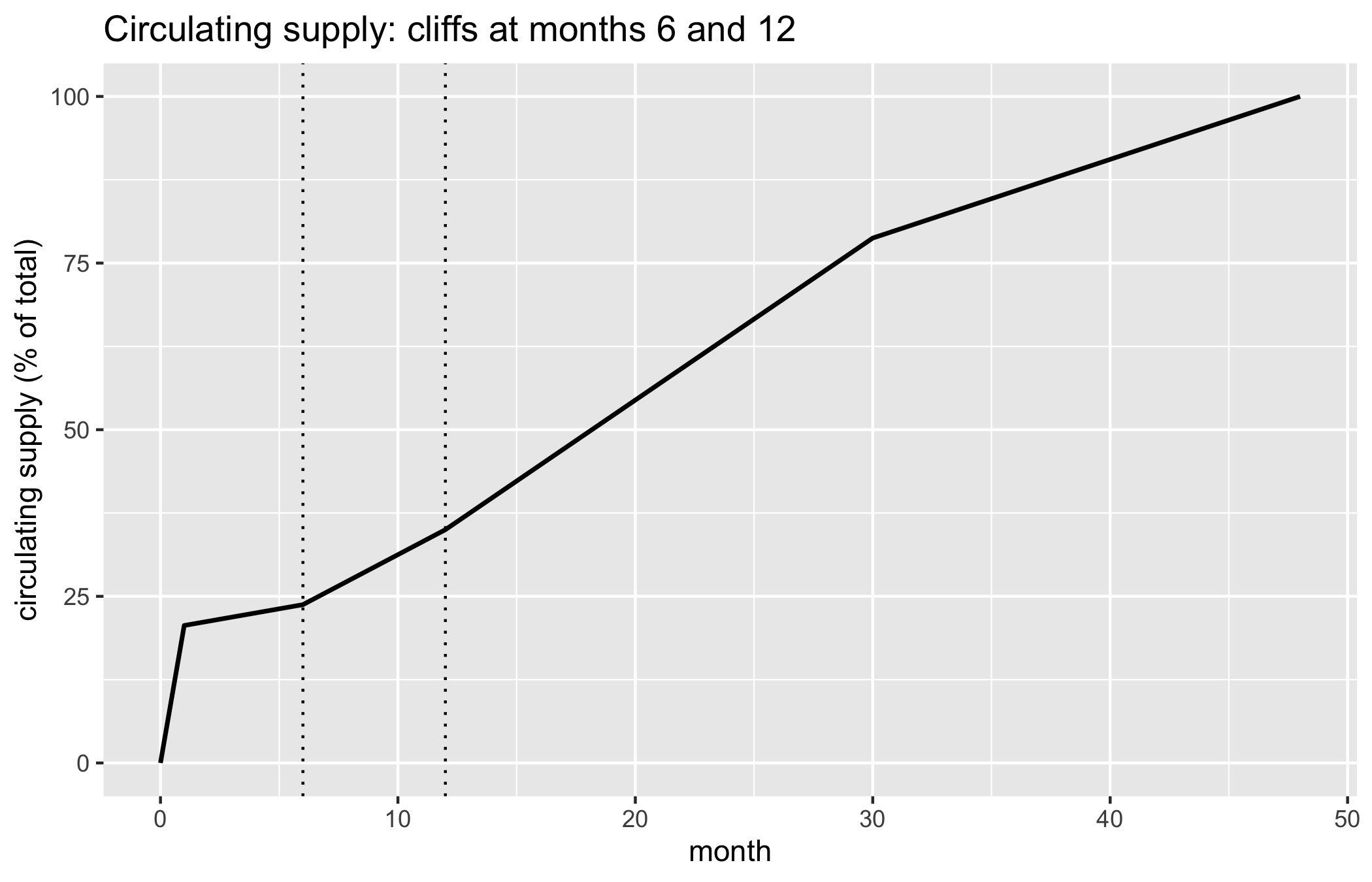
At launch only the public tranche and a sliver of the linear allocations circulate, so market cap is a small fraction of FDV. As the investor cliff at month 6 and the team cliff at month 12 pass, supply climbs toward its full value. A price chart that looks healthy while a large team allocation approaches its cliff is carrying an overhang that market-cap-only reporting hides. The unlock schedule is a tier-one protocol fact, computable today from the vesting contract, and any valuation that ignores it is a tier-four narrative.
Two headline metrics deserve immediate demotion. Market cap, quoted without FDV, hides the unlock overhang and should never be read alone; the honest pair is (market cap, FDV) with the release schedule attached. Total value locked (TVL), the banner statistic of decentralised finance, is a tier-two empirical quantity masquerading as a measure of adoption or safety. TVL is denominated in the very tokens whose prices it aggregates, so it inflates during a bubble by construction; it double-counts value that is rehypothecated, that is, pledged as collateral in one protocol and then re-pledged in another, across protocols; and it says nothing about whether the locked capital can actually exit. A protocol whose TVL doubled because its own token tripled has not become twice as used or twice as safe. Demote both numbers to their tier before quoting them.
11.8.1 Ponzinomics, operationalised
‘Ponzinomics’ is thrown around as an epithet, but it names a precise and testable structure. A scheme is Ponzi-like when the returns paid to existing participants are funded from the capital contributed by new entrants rather than from any exogenous cash flow. But how do we tell a genuine yield from a disguised transfer between cohorts? The operational test follows directly from the definition: we trace the source of the yield. If the protocol produces revenue from outside the token system (trading fees paid by users who want a service, interest paid by borrowers with outside income) the yield has an exogenous source and the scheme is not Ponzi by this test. If the yield is paid in newly minted tokens whose only demand is the expectation of future yield, the source is endogenous and the structure is Ponzi-like: it requires monotonically increasing inflows to sustain the promised return, and it fails when inflows stall.
The test is a flow accounting question, not a moral one, and it is answerable from on-chain data. A statistician can decompose the yield into its funding sources and report the fraction that originates outside the token. The ‘sustainable yield’ narrative becomes a measurable ratio with a value between zero and one, and the closer that ratio sits to zero, the closer the structure sits to a pyramid.
11.8.2 Stablecoin fragility, revisited
The empirical counterpart to this analysis is the stablecoin, a token engineered to hold a fixed value against a reference such as the dollar, studied in detail by Briola et al. (2023), an on-chain and market-microstructure account of a stablecoin collapse. An algorithmic stablecoin that maintains its peg through a reflexive relationship with a companion token, minting one to defend the other, is a Ponzi-like structure with a fixed point that is stable only while inflows grow. The collapse of such a design in May 2022 was a liquidation cascade of exactly the positive-feedback form met in the study of perpetual funding: a small loss of peg triggered redemptions, redemptions minted companion tokens, the new supply drove the companion price down, and the falling companion undermined the very collateral meant to defend the peg. Briola et al. (2023) anatomise the on-chain and market microstructure of the episode, and the lesson for the analyst is that the fragility was visible in the mechanism design before it was visible in the price. A reflexive peg has no exogenous anchor, and the operational Ponzi test would have flagged it.
11.9 Forecasting and calibration
The chapter, and the book, closes by turning the critical lens on the critic. Scepticism is cheap and unfalsifiable unless it commits to predictions and grades them. The instrument, promised in Chapter 1, is a forecasting log scored by the Brier score, the mean squared error between a stated probability and the realised binary outcome. The reader who has followed the COVID-19 forecast-hub literature will recognise both the score and the discipline at once, for scoring a log of crypto predictions is the very exercise by which epidemic forecasters are held to account: a probability, an outcome, and a score, kept prospectively so that the record cannot be edited after the fact.
\[ \text{Brier} = \frac{1}{n} \sum_{i=1}^{n} (p_i - o_i)^2, \qquad o_i \in \{0, 1\}. \]
A forecaster who always says 0.5 scores 0.25, so any score below that is informative and the ideal is zero. But is a low score the same as an honest one? It is not, for a low Brier score alone is not calibration. A forecaster is calibrated when, among all the events assigned probability near \(p\), the long-run frequency of occurrence is \(p\). Calibration is checked by binning predictions and plotting observed frequency against predicted probability: a calibrated forecaster hugs the diagonal.
We exercise the machinery on a SYNTHETIC log of a well-calibrated forecaster, drawing each outcome as a Bernoulli variable at the stated probability, so the calibration curve should track the diagonal up to sampling noise. Replacing this simulated log with a real predictions.csv turns the same code into an assessment of one’s own judgement.
brier_score <- function(prob, outcome) mean((prob - outcome)^2)

set.seed(7)
n <- 200
preds <- tibble(
  prob = runif(n),
  outcome = rbinom(n, 1, runif(n))  # SYNTHETIC: mildly miscalibrated
)
# Force approximate calibration for the demonstration:
preds$outcome <- rbinom(n, 1, preds$prob)

calibration_report <- function(preds, n_bins = 5) {
  overall <- brier_score(preds$prob, preds$outcome)
  binned <- preds |>
    mutate(bin = cut(prob, breaks = seq(0, 1, length.out = n_bins + 1),
                     include.lowest = TRUE)) |>
    group_by(bin) |>
    summarise(n = n(), mean_prob = mean(prob),
              observed = mean(outcome), .groups = 'drop')
  list(brier = overall, binned = binned)
}

rep_out <- calibration_report(preds)
cat('Brier score:', round(rep_out$brier, 4),
    '(0.25 = uninformed coin flip)\n')
#> Brier score: 0.172 (0.25 = uninformed coin flip)

ggplot(rep_out$binned, aes(mean_prob, observed)) +
  geom_abline(linetype = 2) +
  geom_point(aes(size = n)) +
  coord_equal(xlim = c(0, 1), ylim = c(0, 1)) +
  labs(x = 'Predicted probability', y = 'Observed frequency',
       title = 'Calibration of a well-calibrated forecaster')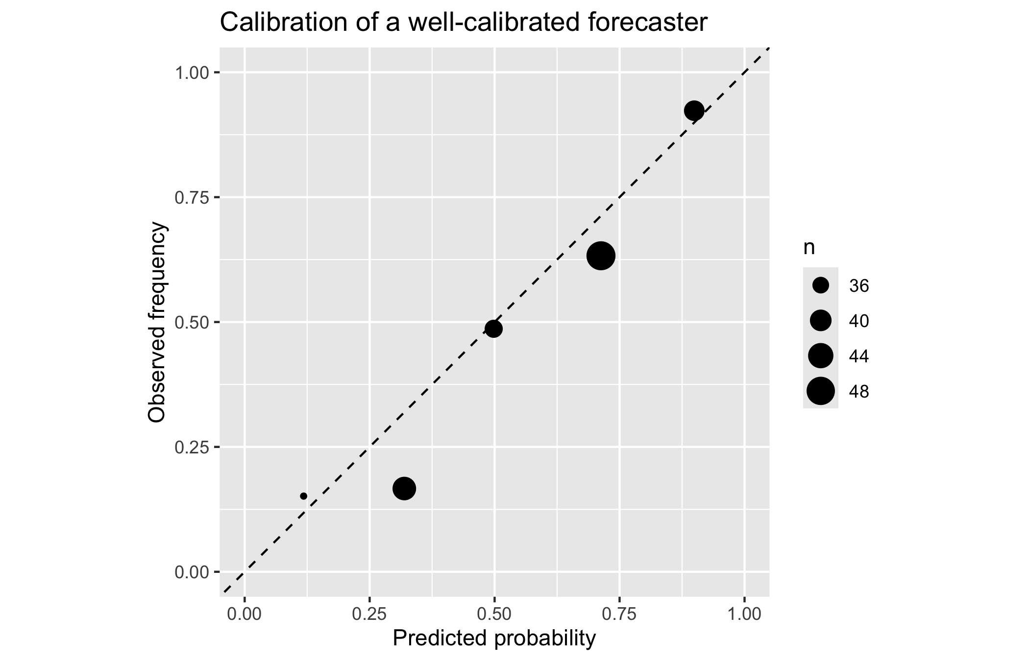
The points hug the diagonal and the Brier score sits well below 0.25, as expected for a forecaster whose probabilities match reality. A real log of crypto predictions will rarely look this clean, which is exactly why one keeps it. The log connects directly to the four falsifiability tiers of Chapter 1. A tier-four narrative cannot be scored, because it names no outcome and no date; forcing a claim into the log is what demotes it to a tier-two empirical statement with a probability, a horizon, and eventually a grade. The discipline is symmetric: it holds the analyst’s scepticism to the same standard it demands of the promoter’s enthusiasm.
A calibration curve earns its keep only by contrast, so we place a second forecaster beside the first. Figure 11.6 draws two SYNTHETIC logs on one reliability plot: a well-calibrated forecaster whose curve tracks the diagonal, and an overconfident one whose curve is too flat, stating extreme probabilities that the outcomes do not earn. The overconfident forecaster is the one to fear, for a strong-sounding prediction is exactly the one a promoter rewards and a careful analyst distrusts.
set.seed(11)
n_cal <- 2000
mk_forecaster <- function(slope) {
  # SYNTHETIC: slope 1 is calibrated; slope < 1 pulls
  # the realised rate toward 0.5, the overconfidence.
  p <- runif(n_cal)
  true_p <- pmin(pmax(0.5 + (p - 0.5) * slope, 0), 1)
  tibble(prob = p, outcome = rbinom(n_cal, 1, true_p))
}
bin_reliability <- function(d, lab, n_bins = 8) {
  d |>
    mutate(bin = cut(prob, seq(0, 1, length.out = n_bins + 1),
                     include.lowest = TRUE)) |>
    group_by(bin) |>
    summarise(mean_prob = mean(prob), observed = mean(outcome),
              .groups = 'drop') |>
    mutate(forecaster = lab)
}
cal_compare <- bind_rows(
  bin_reliability(mk_forecaster(1.0), 'well calibrated'),
  bin_reliability(mk_forecaster(0.5), 'overconfident')
)

ggplot(cal_compare, aes(mean_prob, observed, colour = forecaster)) +
  geom_abline(linetype = 2, colour = 'grey60') +
  geom_line(linewidth = 0.7) +
  geom_point(size = 1.8) +
  scale_colour_manual(values = c('well calibrated' = PAL[1],
                                 'overconfident' = PAL[2])) +
  coord_equal(xlim = c(0, 1), ylim = c(0, 1)) +
  labs(x = 'predicted probability', y = 'observed frequency',
       colour = NULL) +
  book_theme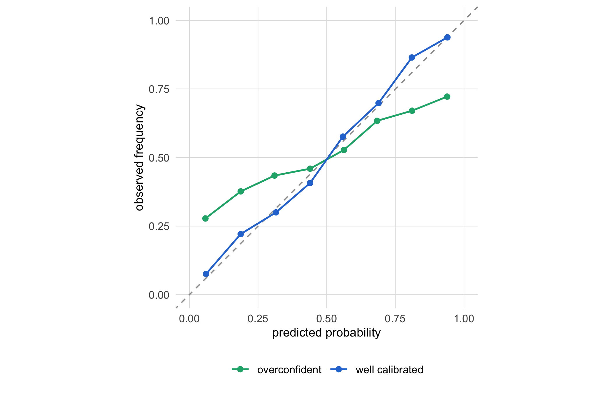
11.10 Worked example: an audit in six numbers
We now assemble the chapter’s instruments into a single pass over one SYNTHETIC chain snapshot, the shape an actual audit would take against a real export. The point is that a handful of numbers, each the output of a familiar statistical tool, summarises the health of a chain more honestly than any dashboard.
set.seed(2026)
# SYNTHETIC snapshot: balances, block intervals, and
# a small forecast log for one chain.
audit_balances <- rlnorm(5000, meanlog = 0, sdlog = 1.9)
audit_intervals <- rexp(1000, rate = 1 / 600)
audit_preds <- tibble(
  prob = runif(50),
  outcome = rbinom(50, 1, runif(50))
)

audit <- tibble(
  metric = c('gini', 'top1pct_share', 'mean_interval_s',
             'ks_p_exponential', 'n_forecasts', 'brier'),
  value = c(
    gini_coef(audit_balances),
    sum(sort(audit_balances, decreasing = TRUE)[1:50]) /
      sum(audit_balances),
    mean(audit_intervals),
    ks.test(audit_intervals, 'pexp',
            rate = 1 / mean(audit_intervals))$p.value,
    nrow(audit_preds),
    brier_score(audit_preds$prob, audit_preds$outcome)
  )
)
audit |> mutate(value = round(value, 4))
#> # A tibble: 6 × 2
#>   metric             value
#>   <chr>              <dbl>
#> 1 gini               0.812
#> 2 top1pct_share      0.301
#> 3 mean_interval_s  640.
#> 4 ks_p_exponential   0.857
#> 5 n_forecasts       50
#> 6 brier              0.327
Read the report honestly. The Gini and top-share quantify concentration, and would be recomputed on clustered entities before any security claim. The mean interval and the KS p-value report whether the block-arrival model holds on this snapshot. The forecast count and Brier score keep the analyst accountable. No single number is a verdict; together they are a defensible, reproducible summary that a reader can rerun and challenge. That reproducibility, every figure regenerated from the code beside it, is the standard the book has tried to hold throughout.
11.10.1 The public-health template
This audit is, line for line, the audit a regulator would run against the trial ledger, or against the vaccine cold-chain provenance log. We verify the integrity commitments, the hash chain of Chapter 1 and Chapter 3, so that the record is known to be tamper-evident. We measure concentration and anomalies, asking whether a handful of sites or actors are responsible for a suspicious share of events. We model the arrival process and report where it departs from expectation, for an unexpected burst of enrolments may be data-entry error or fraud, and an interrupted cold-chain handoff may be a spoiled lot. And we score any predictions the monitoring committee makes, so that oversight is itself calibrated. The statistical toolkit is identical because the underlying question is identical: can this append-only record be trusted, and by how much? A blockchain and a well-kept audit log are two implementations of the same integrity guarantee, and, as Chapter 1 argued, the simpler implementation is usually the right one.
11.11 The right to be forgotten meets the append-only ledger
One tension deserves a section of its own, because it is the point at which this book’s subject matter collides most directly with the law that governs health data. The whole enterprise of the preceding chapters has been to build a record that cannot be altered or deleted. Yet data-protection law presumes the opposite. The European Union’s General Data Protection Regulation grants a right to erasure, and the spirit of health-privacy regimes such as the United States’ HIPAA presumes throughout that personal data can be corrected, restricted, and in the end destroyed. An immutable ledger is engineered precisely so that it cannot honour such a request. Finck states the collision plainly (Finck, 2018): a technology whose value proposition is that nothing can be removed sits uneasily with a body of law whose premise is that the individual may demand removal.
But surely, one might object, a hash or a ciphertext is not personal data, so why not commit those to the chain and keep the plaintext elsewhere? The objection does not survive the machinery of Chapter 3. A hash of a low-cardinality identifier, a national health number or a date of birth, is not anonymisation: it is a commitment that yields to precisely the dictionary attack we ran against the avalanche property, since an adversary who can enumerate the possible inputs can simply hash them all and match. Encryption is stronger, but a key is a secret that can leak, be compelled, or be broken by an advance in capability, and a ledger designed to outlive its participants will still be holding the ciphertext when that day comes. The prudent reading is that anything committed to an immutable ledger should be treated as permanently and potentially publicly disclosed.
The defensible pattern that follows is the one this book has stated wherever the question has arisen: personal health data stays off-chain, in a governed store that can honour an erasure request, and the ledger commits only to non-identifying proofs, a Merkle root (a single hash that commits to an entire dataset) of a locked dataset, a signature over an access grant, a timestamp of an event. The chain then attests that something happened without recording what, to whom, or containing any datum a regulator could later order destroyed.
Under a health-privacy regime, treat the on-chain and off-chain boundary as a hard rule rather than a preference. On-chain: hashes and Merkle roots of locked records, commitments, signatures, and pointers. Off-chain, in an erasable governed store: every datum that identifies a person, and every field a subject could ask to correct or delete. A hash of an identifier is not a safe harbour; it belongs off-chain with the identifier it commits to.
We do not claim the tension is resolved. Reconciling immutability with a right to erasure is an unsettled research question, and the proposed answers, redactable chains built on chameleon hashes that permit an authorised edit, or off-chain storage with on-chain pointers that can be severed, each carry costs and each weaken the very immutability that motivated the ledger. The honest position for a public-health practitioner is that the law here is a binding design constraint and not an afterthought, and that a design which cannot answer ‘how would this honour an erasure request?’ is not yet finished.
11.12 Collaborating with an LLM
On-chain analysis is a domain where a language model accelerates the routine and endangers the inferential. Use it for the first and guard the second.
Prompt. ‘Write R to compute the Gini coefficient and the top-1% share of a vector of account balances, and draw the Lorenz curve, using only base R and ggplot2.’
Watch for: a solution that pulls in ineq or DescTools when the closed form is four lines; an off-by-one in the rank weighting of the Gini formula; a Lorenz curve that omits the origin point and so understates the area.
Verification: check the Gini against a known case (perfect equality gives 0, one holder gives near 1) and confirm the Lorenz curve starts at (0, 0) and ends at (1, 1).
Prompt. ‘Here is a description of a token’s staking rewards. Is the yield sustainable?’
Watch for: a confident narrative verdict with no flow accounting. The model will happily echo the project’s own framing.
Verification: insist on the operational test. Trace the yield to an exogenous or endogenous source, and demand the on-chain quantity that would distinguish them. A verdict without a funding decomposition is a tier-four opinion.
Prompt. ‘Fit an exponential to these block intervals and tell me if it is a good model.’
Watch for: a single KS p-value reported as a verdict, with no attention to serial dependence or to the retarget and hash-shock regimes where the model is expected to fail.
Verification: require the QQ plot and an explicit statement of where the fit is weakest. A high p-value on the pooled data is consistent with severe misfit in exactly the stress episodes that matter.
11.13 Exercises
Estimand audit. Take a published on-chain metric (daily active addresses, TVL, or realised capitalisation) and write one paragraph naming its estimand, the ledger quantity actually measured, and the selection, confounding, and measurement gaps between them.
Gini sanity checks (quantitative). Prove that the closed-form
gini_coefreturns 0 for a perfectly equal population and approaches \((n-1)/n\) when one holder owns everything. Verify both limits numerically, and confirm the estimator is scale-invariant.Lorenz and concentration (quantitative). Simulate balances from a Pareto distribution with tail index \(\alpha \in \{1.5, 2.0, 2.5\}\). For each, compute the Gini and the top-1% share and overlay the three Lorenz curves. Relate the direction of the change in Gini to the change in \(\alpha\), and explain the mechanism.
Entity versus address Gini (quantitative). Extend the union-find clustering to attach a balance to each address, then compute the Gini on addresses and on the resulting entities for the same synthetic chain. Construct one scenario where clustering raises the Gini and one where it lowers it, and state which is the security-relevant number.
Where the exponential breaks (quantitative). Simulate block intervals with a rate that steps up by 50% halfway through the series (a hash-rate shock). Fit a single exponential to the pooled data, report the KS p-value, and show via the QQ plot and a plot of intervals over time that the pooled test can fail to detect a regime it visibly contains.
Ponzi flow test. Design a schema for the minimal on-chain quantities you would need to compute the fraction of a protocol’s yield that originates from exogenous revenue. State the decision rule that would classify the yield as Ponzi-like, and name one way the schema could be gamed.
11.14 Further reading
Meiklejohn et al. (2013) is the foundational de-anonymisation paper: read it for the heuristics and for the demonstration that pseudonymity degrades under patient analysis. Kondor et al. (2014) gives the empirical wealth-concentration study whose Lorenz and Gini analysis this chapter reproduces on synthetic data. Briola et al. (2023) anatomise a stablecoin collapse with on-chain and microstructure data, the empirical case for the reflexive-peg fragility discussed here.
For quantitative treatments of the wider field, Goffard (2023) collects probabilistic and statistical models of blockchain phenomena, and the two systematisation-of-knowledge papers, Bonneau et al. (2015) on Bitcoin and cryptocurrencies and Werner et al. (2022) on decentralised finance, map the research landscape and its open problems with more rigour than any promotional source. Narayanan et al. (2016) remains the reference textbook, and its final chapters on anonymity and community are the natural sequel to this one.
11.15 Synthesis: achievements, theatre, and calibration
We began the book with a claim that a blockchain is an append-only ledger that mutually distrusting parties agree on without a trusted intermediary, and that this one sentence contains the entire subject. Ten weeks later the sentence has been made quantitative at every clause. The consensus is a random walk and a cost-of-attack calculation. The cryptography is a measurable set of statistical properties. The economics is a collection of control systems and feedback loops. And the data, as this chapter has shown, is an observational dataset to be analysed with the ordinary and powerful instruments of the trade, the same instruments we bring to a registry or a trial.
What remains is judgement, and judgement divides the genuine from the theatrical. The genuine achievement is real and difficult, namely open-membership Byzantine agreement without a trusted party, a problem Lamport et al. (1982) posed and Nakamoto (2008) answered, delivering a tamper-evident record whose integrity a health scientist has good reason to want. The theatre is also real, in the unfalsifiable valuations, the metrics engineered to impress, and the reflexive schemes that dress a pyramid in the vocabulary of finance. On the one hand a credulous enthusiasm mistakes the theatre for the achievement; on the other, a reflexive dismissal throws out the achievement with the theatre. A calibrated analyst holds both without collapsing into either, and the instruments that keep the two apart are the ones on which this chapter and this book have ended.
In conclusion, three points are to be emphasized. First, a public chain is an observational dataset and must be read as one, with the estimand named before the estimator and the selection, confounding, and measurement gaps between the ledger and the latent quantity stated in the open; every instrument in this chapter, from the Gini coefficient to the capture-recapture logic of address clustering, has a public-health twin, and the honesty demanded of a registry analysis is demanded here without relaxation. Second, pseudonymity is not anonymity, neither on a chain nor in a registry, and because an append-only store never forgets, the re-identification risk of pseudonymised health data written to a public ledger grows rather than decays with time; this is a decisive argument for keeping patient-level records off any public chain and for confining the trial ledger to integrity commitments alone. Third, scepticism that is never recorded is merely a posture, and the remedy is to name the falsifiability tier of every claim, to operationalise each narrative into a test with a rejection region, and to keep a prospectively scored forecasting log so that the analyst’s own judgement is calibrated against outcomes by the same Brier score demanded of the epidemic forecaster and the promoter alike. A blockchain and a well-kept audit log are, in the end, two implementations of one integrity guarantee, and, as we argued in Chapter 1, the simpler implementation is usually the right one. That principle, and not any enthusiasm for the technology, is what we hope the reader carries forward.