In the original Bitcoin paper, it was suggested that the blockchain arrivals occur according to a homogeneous Poisson process.
Bowden, Keeler, Krzesinski, and Taylor, Block Arrivals in the Bitcoin Blockchain (2018)
5.1 Learning objectives
By the end of this chapter the reader should be able to:
Derive block discovery as a Poisson process from tiny-probability Bernoulli hashing, and state precisely why block inter-arrival times are exponential.
Fit the geometric model for attempts-to-success and confirm that mean work scales as \(16^{\text{difficulty}}\).
Analyse the difficulty retarget rule as a discrete-time feedback controller acting on a stochastic input, and predict its transient response to a hash-power shock.
Estimate the orphan (fork) rate from the mean block time and a propagation window, and explain why shorter target intervals mechanically raise it.
Estimate current hash rate from observed block timestamps, with an interval that reflects the exponential sampling variability.
Name the failure modes of the simple exponential model on real chains.
5.2 Orientation
We begin with an observation that should reassure the reader. A biostatistics student who has fit an exponential survival model, and an epidemiologist who has watched Poisson counts accumulate on a disease-surveillance system, already command every tool this chapter requires. The reason is simple to state: block arrivals are arrival data. A block discovered on a chain is an event in continuous time, the interval between two consecutive blocks is a waiting time, and the stream of such events is a point process of precisely the kind one meets in survival analysis and in the surveillance of incident cases. Nothing in the machinery below is foreign to a reader trained on time-to-event outcomes; it is a familiar subject presented in unfamiliar terms.
The public-health problem that motivates the chapter is one of settlement timing. The running case study of this book is a multi-institution clinical-trial data-integrity ledger, which we shall refer to henceforth as the trial ledger. Several hospitals share an append-only record of enrolment, randomisation, and outcome events, no single institution is trusted to hold the master copy, and a regulator audits the record after the fact. The record advances only as fast as blocks are appended to it, so the arrival stream that this chapter studies is exactly what governs how quickly a randomisation becomes irrevocably committed and how long an auditor must wait before a record may be treated as settled. A vaccine cold-chain provenance system, in which each custody handoff of a temperature-sensitive consignment is written to a shared ledger, furnishes a secondary example with the same arrival-time character. In both, the question ‘how long until this record is safe to rely upon?’ is a question about block inter-arrival times, and it is a statistical question.
Seen this way, mining is not, at its core, a cryptographic puzzle. It is a stochastic process observed through a control system. A miner performs an enormous number of near-independent trials, each with a vanishingly small success probability, and the resulting arrival stream of blocks is a Poisson process whose rate the protocol holds fixed by feedback. Every object in this description is one the reader already owns: Bernoulli trials, the geometric and exponential waiting-time laws, superposition of Poisson processes, memorylessness, and a proportional controller correcting a noisy plant.
NoteThe vocabulary of this chapter
The statistical terms below will be familiar to a reader trained in survival analysis; we state them here in the arrival-time language this chapter uses, alongside the few terms specific to mining.
Bernoulli trial and the geometric distribution. A Bernoulli trial is a single success-or-failure experiment with fixed success probability \(p\); one hashing attempt is such a trial. The geometric distribution is the law of the number of trials needed to obtain the first success, with mean \(1/p\); here it counts the hashes a block costs.
Exponential distribution and memorylessness. The exponential is the continuous waiting-time law with a constant hazard, meaning that the chance of an event in the next instant does not depend on how long one has already waited. This ‘memoryless’ property is the survival-analysis constant-hazard assumption, and it makes the wait for the next block indifferent to past failures.
Poisson process and superposition. A Poisson process is a stream of events in continuous time whose counts in disjoint windows are independent Poisson variables and whose gaps are exponential; it is the standard model for events arriving at random, as in disease surveillance. Superposition is the fact that merging several independent Poisson processes yields one Poisson process whose rate is the sum of the parts, which is how many independent miners combine into a single arrival stream.
Hash rate. The number of hashing attempts a miner, or the whole network, performs per second. It sets the block-arrival rate and is not published by the chain, so it must be estimated.
Difficulty retarget. The rule by which the protocol periodically rescales the mining difficulty, and hence the per-attempt success probability, so as to hold the mean interval between blocks at a fixed target.
Feedback controller and set point. A feedback controller is a rule that measures a system’s output, compares it with a desired value called the set point, and adjusts an input to reduce the discrepancy. The retarget is such a controller, with the ten-minute mean interval as its set point.
Orphan (or fork) rate. The fraction of mined blocks that are discarded because two miners found a block at nearly the same time and the network eventually kept only one. A discarded block is called an orphan or stale block.
Quantile-quantile (QQ) plot. A diagnostic that plots the ordered observed values against the quantiles a fitted distribution predicts; points on the diagonal indicate agreement in distribution, and systematic departure signals that the assumed law is wrong.
The identification with event and arrival data is exact, and we shall exploit it in line rather than reserve it for a closing remark. A block inter-arrival time is an exponential waiting time, so the memoryless property is the constant-hazard assumption, a drifting arrival rate is a time-varying hazard, and the quantile-quantile plots and goodness-of-fit tests we shall apply are the very diagnostics one uses to check an exponential survival fit. The transfer runs in both directions: the mining chain is a concrete, fully observed point process on which to rehearse methods whose biomedical applications, in surveillance and in trials, are noisier and harder to validate.
We proceed constructively. We first establish the Poisson structure, then measure it in R on a toy chain whose hashing is genuine. We fit the geometric law of attempts and read its diagnostics as survival diagnostics; we develop a worked surveillance analogy and note carefully where it ends; we treat difficulty adjustment as a controller and watch it absorb a doubling of hash power; then we derive a fork-rate estimate and a hash-rate estimator. We close by asking where the tidy exponential model breaks on real chains, because that boundary, whether on a chain or in a surveillance stream, is where the interesting science resides.
5.3 The statistician’s contribution
Three judgements sit at the centre of this chapter, and it merits emphasis that none of them is automated by any mining tool or block explorer. Each is a modelling act of the sort a biostatistician performs when deciding how to treat a stream of adverse-event or incidence times.
Recognising the renewal and Poisson structure. A renewal process is one in which the waiting-time clock restarts afresh after each event, so the gaps are independent and identically distributed. Seeing that independent tiny-probability hashing produces a Poisson arrival process, and therefore that inter-arrival times are exponential and memoryless, is what licenses every downstream calculation: the waiting-time law, the superposition of many miners into one aggregate process, and the fork rate. Nothing about the source code announces this; it is a modelling act.
Treating difficulty as a controller, not a constant. The retarget rule is a discrete-time feedback controller acting on a stochastic input. Framing it that way turns vague questions (‘will block times recover after a hash-power surge?’) into precise ones about transient response, stability, and oscillation, answerable with the tools of control theory rather than intuition, following Kraft, who analysed the retarget rule as a control problem (Kraft, 2016).
Knowing the exponential model’s failure modes. The memoryless model is exact under constant hash rate and instantaneous propagation, and it frays predictably when those assumptions fail: propagation delay, non-constant hash rate across a retarget epoch, and deviations documented on real chains by Bowden and colleagues, who modelled Bitcoin block-arrival times and identified where the simple Poisson model fails (Bowden et al., 2020). A statistician’s value is as much in stating where the model stops holding as in fitting it.
5.4 Block discovery as a Poisson process
We begin with the generating mechanism. Fix a difficulty and let \(H(\cdot)\) be the hash function. A single hashing attempt succeeds when its digest falls below the target, an event of probability \(p\). In our toy model the target is a prefix of \(d\) hexadecimal zeros, so \(p = 16^{-d}\), because each hex digit takes \(16\) equally likely values and \(d\) of them must be zero. Attempts are, for all practical purposes, independent Bernoulli\((p)\) trials with \(p\) minuscule.
From this modest premise three classical facts follow immediately.
The number of attempts until the first success is Geometric\((p)\), with mean \(1/p = 16^{d}\). This is the number of hashes one block costs.
A miner performing hashes at rate \(r\) per second therefore finds blocks at rate \(\lambda = r p\) per second. Because \(p\) is tiny and \(r\) is huge, the discrete geometric count is indistinguishable from a continuous exponential waiting time: the time to the next block is Exponential\((\lambda)\), with mean \(1/\lambda\).
If many miners hash independently at rates \(r_1, r_2, \dots\), their block discoveries superpose into a single Poisson process of rate \(\lambda = p \sum_i r_i\), proportional to total hash power. The identity of the finder is an independent multinomial draw with probabilities \(r_i / \sum_j r_j\).
It helps to hold the whole correspondence in view at once. Every object in the mining process carries a distribution and an exact public-health twin, together with the diagnostic one reaches for to check it (Table 5.1).
Table 5.1: The mining distributions and their public-health twins
Object
Distribution
Public-health twin
Diagnostic
Single hash attempt
Bernoulli\((p)\)
Event indicator
n/a
Attempts to success
Geometric\((p)\)
Trials to first event
Geometric QQ
Waiting time to next block
Exponential\((\lambda)\)
Survival time under constant hazard
Exponential QQ, KS
Arrivals in a window
Poisson\((\lambda w)\)
Surveillance case counts
Dispersion check
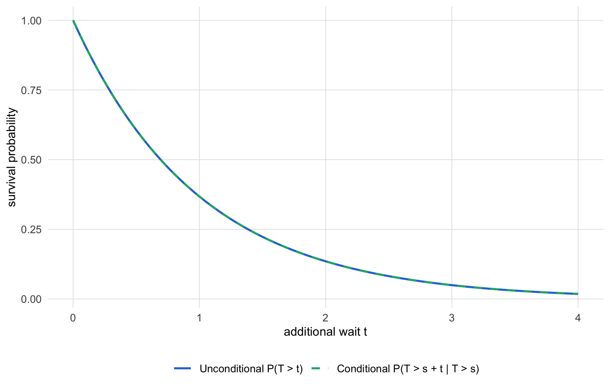
The decisive property is memorylessness. Having hashed for an hour without success leaves the distribution of the remaining wait unchanged: the process has no notion of being ‘due’. A miner who has found nothing all day is in exactly the position of one who just started. This is the mining folklore ‘hashing has no memory’ stated as the defining property of the exponential law, \(P(T > s + t \mid T > s) = P(T > t)\). The reader will recognise it at once as the constant-hazard assumption of survival analysis: a memoryless waiting time is precisely one whose hazard does not depend on how long we have already waited, and the exponential is the unique continuous law with that property.
The claim is worth seeing rather than only stating. If we plot the survival curve of a fresh wait and, on the same axes, the survival curve of the remaining wait given that a period \(s\) has already elapsed without success, the two lie exactly on top of one another (Figure 5.1). Waiting confers no advantage.
Figure 5.1: The survival curve of a fresh exponential wait and the survival curve of the remaining wait, given that a period has already elapsed without success, coincide exactly; this is the memoryless property that makes mining a constant-hazard process.
We measure this on a toy chain whose hashing is genuine SHA-256. The mining primitive below is the one from Chapter 4, reused verbatim: it increments a nonce (a counter varied to change the hashed input) until the digest (the hash output) carries the required prefix, and records the attempt count.
We now put the geometric prediction to the test. We harvest per-block attempt counts at two difficulties and compare them with theory. Attempts to mine one block are Geometric with success probability \(p = 16^{-d}\), so the mean is \(16^{d}\).
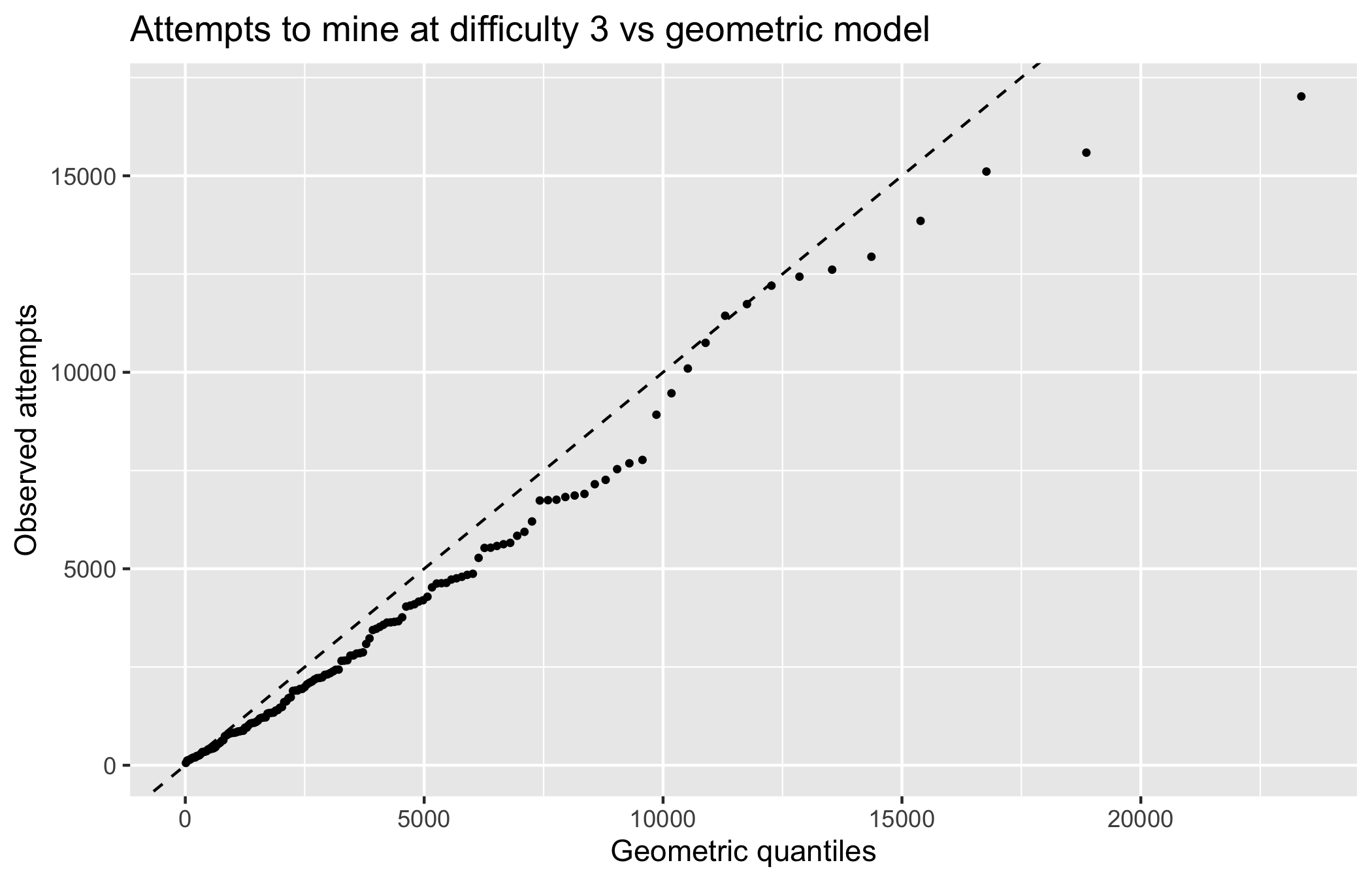
The observed mean attempts track \(16^{d}\), and the ratio between difficulties 3 and 2 lands near 16: the quantitative content of ‘one more hex zero costs sixteen times the work’. But agreement in the mean is a weak test, and a natural question arises. Does the whole distribution match, or have we confirmed only its first moment? A quantile-quantile plot against the geometric law settles the point, confirming the distributional form and not merely the mean.
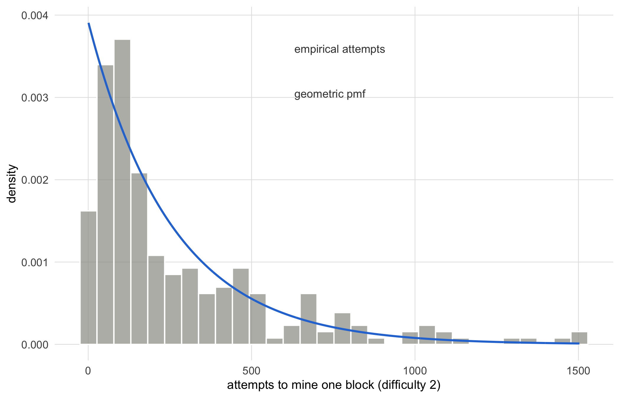
We can look even more directly first. Overlaying the geometric mass function on the difficulty-2 attempt counts already in hand shows the whole shape, and not only the mean, before we turn to the more sensitive quantile-quantile view (Figure 5.2).
p2<-16^(-2)kk<-seq_len(max(a2))pmf<-tibble::tibble(k =kk, d =dgeom(kk-1, prob =p2))maxd<-dgeom(0, p2)ggplot()+geom_histogram( data =tibble::tibble(a =a2),aes(a, after_stat(density)), bins =30, fill ='#9a9a92', colour ='white', alpha =0.7)+geom_line(data =pmf, aes(k, d), colour =PAL[1], linewidth =0.8)+annotate('text', x =0.42*max(a2), y =0.92*maxd, label ='empirical attempts', colour ='grey25', hjust =0, size =3.2)+annotate('text', x =0.42*max(a2), y =0.78*maxd, label ='geometric pmf', colour ='grey25', hjust =0, size =3.2)+book_theme+labs(x ='attempts to mine one block (difficulty 2)', y ='density')
Figure 5.2: The distribution of attempts to mine one block at difficulty 2, overlaid with the geometric mass function it should follow; agreement across the whole shape, not merely at the mean, is what licenses the geometric model.
Figure 5.3: Attempts-to-mine at difficulty 3 against the geometric model. Points on the diagonal indicate agreement in distribution, not only in mean.
It merits emphasis that the diagnostic is not an analogue of a survival-analysis tool; it is the same tool. The quantile-quantile plot a biostatistician draws to check whether censored survival times follow an assumed law is doing the work here, applied to a mining process in place of a time-to-event outcome. Points on the diagonal license the distributional assumption; systematic departure from it, in either setting, is the signal that the assumed law is wrong.
NoteCheck your understanding: memorylessness and the 16-fold cost
A miner has hashed for what would be, on average, half a block’s worth of work at difficulty 3 without finding a block. Is the expected remaining work now \(16^3 / 2\)? Separately, why does adding one hex zero to the target multiply the expected work by exactly 16?
The expected remaining work is still the full \(16^3\), not half. Attempts are independent Bernoulli trials, so the count to the next success is memoryless (geometric); past failures carry no information about how much longer the wait will be. The 16-fold cost follows because requiring one more leading hex zero divides the set of valid targets by 16, so \(p\) falls from \(16^{-d}\) to \(16^{-(d+1)}\) and the mean \(1/p\) rises by a factor of 16.
5.6 Difficulty adjustment as feedback control
Block intervals are exponential with mean difficulty divided by hash rate. If total hash rate changes, the mean interval changes in inverse proportion, and the protocol must move difficulty to hold the mean at its set-point (ten minutes on Bitcoin). But how does a protocol with no central operator hold a mean arrival rate fixed against a fluctuating and adversarial input? The retarget rule is the answer: every epoch (2016 blocks on Bitcoin) it scales difficulty by the ratio of observed mean interval to target,
Kraft (Kraft, 2016) analyses precisely this rule as a control problem, and it is the framing we adopt: the retarget is a discrete-time feedback controller acting on a stochastic plant. The control action is applied once per epoch, not continuously, so the loop has a built-in dead time (a delay before any correction can take effect): a change in hash rate is uncorrected until the next retarget.
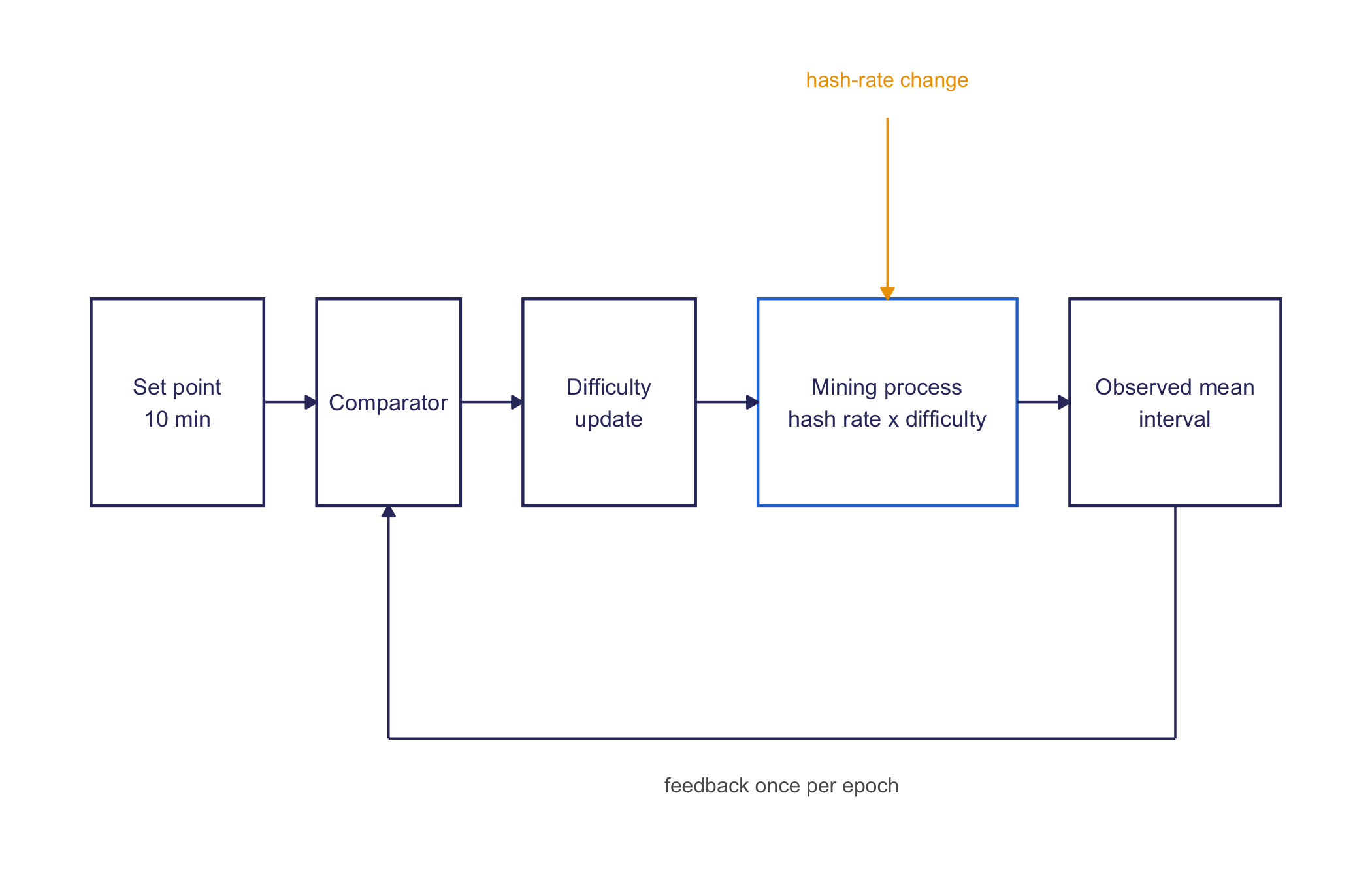
It is worth drawing the loop before analysing it. Read as a block diagram, the retarget is an ordinary negative-feedback controller with five parts: a set point, a comparator, an update rule, a stochastic plant, and a measured output fed back to the comparator (Figure 5.4).
box<-tibble::tibble( label =c('Set point\n10 min', 'Comparator','Difficulty\nupdate','Mining process\nhash rate x difficulty','Observed mean\ninterval'), xc =c(1.2, 3.4, 5.7, 8.6, 11.6), hw =c(0.9, 0.75, 0.9, 1.35, 1.1))box$xmin<-box$xc-box$hwbox$xmax<-box$xc+box$hwbox$ymin<-2.4box$ymax<-3.2box$border<-c('#33356b', '#33356b', '#33356b',PAL[1], '#33356b')fwd<-tibble::tibble( x =box$xmax[1:4], xend =box$xmin[2:5])ggplot()+geom_rect(data =box,aes(xmin =xmin, xmax =xmax, ymin =ymin, ymax =ymax), fill ='white', colour =box$border, linewidth =0.5)+geom_text(data =box, aes(xc, (ymin+ymax)/2, label =label), size =2.9, colour ='#33356b')+geom_segment(data =fwd, aes(x =x, xend =xend), y =2.8, yend =2.8, colour ='#33356b', linewidth =0.4, arrow =arrow(length =unit(0.16, 'cm'), type ='closed'))+geom_segment(aes(x =box$xc[5], y =2.4, xend =box$xc[5], yend =1.5), colour ='#33356b', linewidth =0.4)+geom_segment(aes(x =box$xc[5], y =1.5, xend =box$xc[2], yend =1.5), colour ='#33356b', linewidth =0.4)+geom_segment(aes(x =box$xc[2], y =1.5, xend =box$xc[2], yend =2.4), colour ='#33356b', linewidth =0.4, arrow =arrow(length =unit(0.16, 'cm'), type ='closed'))+geom_segment(aes(x =box$xc[4], y =3.9, xend =box$xc[4], yend =3.2), colour =PAL[3], linewidth =0.4, arrow =arrow(length =unit(0.16, 'cm'), type ='closed'))+annotate('text', x =box$xc[4], y =4.05, label ='hash-rate change', size =2.7, colour =PAL[3])+annotate('text', x =(box$xc[5]+box$xc[2])/2, y =1.32, label ='feedback once per epoch', size =2.7, colour ='grey35')+coord_cartesian(xlim =c(0, 13), ylim =c(1.1, 4.2), clip ='off')+theme_void()
Figure 5.4: Difficulty adjustment read as a discrete-time feedback loop: the observed mean interval is compared with the ten-minute set point, the difficulty update responds once per epoch, and the mining process turns hash rate and difficulty into the next interval, so a hash-rate change is corrected only at the following retarget.
The reader with a trials background will find the mechanism intuitive, for it is an adaptive procedure of a familiar kind. A retarget re-estimates a nuisance quantity, the effective hash rate, from the data accumulated over an epoch, and adjusts a design parameter, the difficulty, so as to hold a target quantity, the mean arrival rate, at its set-point. The construction has the same shape as an adaptive clinical-trial design that re-estimates the sample size at an interim analysis when the observed nuisance variance departs from the value assumed at planning. In both cases one looks at accumulating data, updates an estimate of something one does not control, and moves a lever to keep an operating characteristic on target.
We should be careful, however, to mark where the analogy ends, for it ends at an important place. The retarget acts on the generating rate itself: raising the difficulty makes blocks physically harder to find and so slows their true arrival. Adaptive sample-size re-estimation, by contrast, acts only on the sampling plan, that is, on how many patients are enrolled or how long they are followed; it does not, and could not, alter the underlying event rate of the disease. The mining controller reaches into the data-generating process; the trial design reaches only into the observation process. This distinction is not a quibble. It is the reason a difficulty retarget can erase a rate change entirely, whereas an adaptive trial design must live with whatever event rate nature supplies.
Before simulating the transient, we can tabulate what a doubling of hash power moves, and what the retarget subsequently restores (Table 5.2).
Table 5.2: What a doubling of hash power moves, before and after the retarget
Quantity
Before retarget
After retarget
Per-hash success probability
Unchanged; set by difficulty, not power
Halved, as difficulty doubles
Expected block interval
Halved, near five minutes
Restored to ten minutes
Interval variance
Quartered; varies as the squared mean
Restored
Orphan rate (\(\approx \Delta / \mu\))
Doubled
Restored to baseline
We now simulate an instantaneous doubling of hash power and watch the controller correct. But how quickly, and how smoothly, does the mean interval return to its set-point? The epoch is shortened to 40 blocks for illustration; the real Bitcoin epoch is 2016.
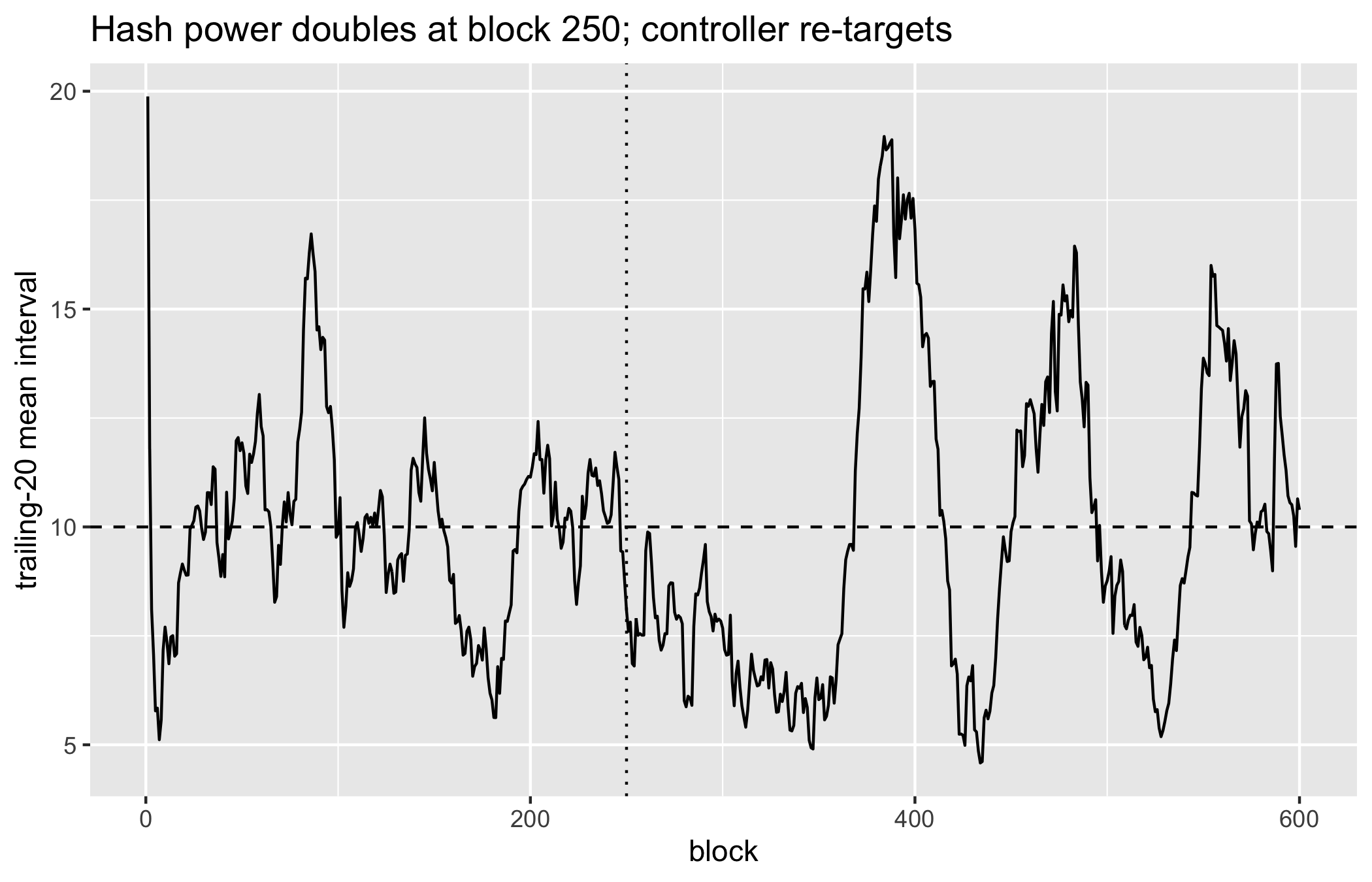
trailing_mean<-function(x, k){vapply(seq_along(x),function(i)mean(x[max(1, i-k+1):i]),numeric(1))}simulate_retarget<-function(n=600, target=10,epoch=40,shock_at=250){hashrate<-1difficulty<-targetinterval<-numeric(n)for(iinseq_len(n)){if(i==shock_at)hashrate<-2*hashrateinterval[i]<-rexp(1, rate =hashrate/difficulty)if(i%%epoch==0){recent<-mean(interval[(i-epoch+1):i])difficulty<-difficulty*target/recent}}tibble::tibble(block =seq_len(n), interval =interval)}set.seed(5)sim<-simulate_retarget()sim$roll<-trailing_mean(sim$interval, 20)ggplot(sim, aes(block, roll))+geom_line()+geom_hline(yintercept =10, linetype =2)+geom_vline(xintercept =250, linetype =3)+labs(x ='block', y ='trailing-20 mean interval', title =paste('Hash power doubles at block','250; controller re-targets'))
Figure 5.5: The difficulty controller absorbs a doubling of hash power at block 250. Blocks briefly arrive twice as fast (trailing mean near five), then the next retarget restores the ten-block set-point.
Immediately after the shock the trailing mean drops toward five, because blocks arrive twice as fast at the old difficulty, then the next retarget roughly doubles difficulty and pulls the mean back to ten. This is the negative-feedback dynamics of any proportional controller, and it explains why a permanent change in global hash rate produces only a transient change in block time.
The controller is stable but not free of oscillation. Because it corrects on the mean of a noisy epoch and acts with a one-epoch lag, an over-correction can overshoot in the following epoch, and the standard rule’s damping (Bitcoin clamps the per-epoch adjustment to the interval \([1/4, 4]\)) exists precisely to bound this oscillation. A statistician recognises the classic tension between a controller aggressive enough to track real changes and cautious enough not to chase sampling noise.
ImportantThe sceptic’s reflex
A recurring claim is that mining difficulty ‘always rises’. Name the tier before believing it. This is an empirical claim about the past, not a protocol fact about the future. The retarget rule is symmetric: it lowers difficulty exactly as readily as it raises it, and difficulty has fallen materially in every sustained hash-rate decline (for instance after large regional miner shutdowns). The monotone-rise story is a narrative extrapolated from a bull-market regime, and the controller’s own definition falsifies it. What the protocol guarantees is regulation toward the target interval, not a monotone difficulty path.
5.7 A surveillance reading of the same mathematics
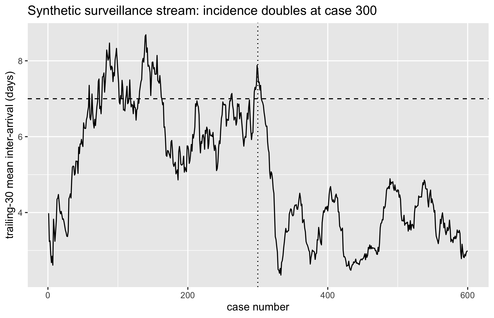
To make the epidemiologic identification concrete, rather than merely asserted, we develop it as a worked example. Consider a disease-surveillance system that records the time of each incident case reported to a health department. Under a stable incidence the reports arrive as a Poisson process, so the inter-arrival gaps between successive cases are exponential, and the analyst’s first task is exactly the one performed above for blocks: fit the rate and check the exponential assumption with a quantile-quantile plot and a goodness-of-fit test. An outbreak is an increase in the arrival rate, and detecting it is the surveillance counterpart of detecting a hash-rate shock. To illustrate, consider a synthetic record of six hundred cases in which the incidence doubles midway through, at case three hundred.
set.seed(72)# SYNTHETIC: case inter-arrival gaps in days. Baseline# incidence gives a mean gap of 7 days; an outbreak at# case 300 doubles the rate, halving the mean gap.baseline<-rexp(300, rate =1/7)outbreak<-rexp(300, rate =2/7)case_gap<-c(baseline, outbreak)surveil<-tibble::tibble( case =seq_along(case_gap), roll =trailing_mean(case_gap, 30))ggplot(surveil, aes(case, roll))+geom_line()+geom_hline(yintercept =7, linetype =2)+geom_vline(xintercept =300, linetype =3)+labs(x ='case number', y ='trailing-30 mean inter-arrival (days)', title =paste('Synthetic surveillance stream:','incidence doubles at case 300'))
Figure 5.6: SYNTHETIC disease-surveillance case arrivals. A doubling of incidence at case 300 halves the trailing-mean inter-arrival gap. Unlike the mining chain, no controller restores the set-point: in surveillance the rate change is the signal we wish to detect, not a disturbance to reject.
The trailing-mean gap halves at the change-point, in the same manner as the trailing-mean block interval dropped after the hash-power shock. It merits notice that a marginal test on the pooled record is relatively insensitive here, because a fifty-fifty mixture of two exponentials remains roughly exponential in its unordered distribution, so a quantile-quantile plot or a Kolmogorov-Smirnov test (a goodness-of-fit test comparing an empirical distribution with a hypothesised one) applied to all six hundred gaps at once may fail to reject. The change is a sequential phenomenon, not a marginal one, and it is visible only when the data are read in arrival order. This is the same lesson a survival analyst learns from an unmodelled change-point in the hazard: pooling across the change hides it, and a time-ordered or change-point analysis is required to recover it.
Here the two settings part company, and the parting is instructive. The mining protocol treats a rate change as a disturbance and deploys the retarget controller to erase it, returning the mean interval to its set-point. The surveillance analyst treats the identical rate change as the quantity of interest and wishes above all to detect it, quickly and with controlled false-alarm rate. The mathematics of the arrival process is common to both; what differs is whether the change is a nuisance to be regulated away or a finding to be reported. The reader designing an alarm rule for the trial ledger, in which an unexpected surge of outcome events written across several hospitals might signal a safety problem, sits on the surveillance side of this divide and not the controller side.
5.8 Fork and orphan rate
Two miners can find a block at nearly the same height before either has heard of the other. When the network converges on one, the other becomes an orphan (or stale) block. This is not an academic concern for the trial ledger: a randomisation event written into a block that is later orphaned appears, for a short interval, to be committed and then is reorganised out of the accepted history, which is precisely why an auditor must wait a number of confirmations before treating a record as settled. How often, then, does such a competing block occur? Under the Poisson model the rate is a short calculation, and Decker and Wattenhofer, who measured block propagation in the live Bitcoin network, ground it in observed delays (Decker & Wattenhofer, 2013). Let \(\mu\) be the mean block time, so blocks arrive as a Poisson process of rate \(\lambda = 1/\mu\), and let \(\Delta\) be the propagation window: the time for a newly found block to reach the rest of the network. A fork occurs when a competing block is found within \(\Delta\) of a given block. By the memoryless property, the wait to the next block is Exponential\((\lambda)\), so
for \(\Delta \ll \mu\). The approximation is the statement that matters: the orphan rate is, to first order, the propagation window measured in units of the mean block time. Below we compute it across regimes and confirm the closed form by simulating exponential inter-arrival gaps and counting those shorter than the window.
The simulated column tracks the closed form to Monte Carlo noise. Read down the table: holding the propagation window fixed, shrinking the mean block time from 600 seconds to 15 raises the orphan rate by roughly the same factor, because the rate is approximately \(\Delta / \mu\). This is the mechanical cost of fast blocks. A chain that targets short intervals to appear ‘fast’ spends a larger fraction of its work on blocks that lose the fork race, which both wastes hash power and weakens security, since orphaned work does not defend the chain. The propagation window \(\Delta\) is a network property that no protocol parameter can eliminate, so it sets a floor on the block time below which orphan rates become costly.
NoteCheck your understanding: why fast blocks fork more
A chain proposes to cut its target block time from ten minutes to one minute to improve user experience, keeping the same peer-to-peer network and therefore the same propagation window \(\Delta\). Roughly what happens to the orphan rate, and why is this a security concern and not merely a bandwidth one?
The orphan rate scales approximately as \(\Delta / \mu\), so cutting \(\mu\) by a factor of ten raises the orphan rate by roughly ten. It is a security concern because work spent on orphaned blocks does not contribute to the longest chain: an honest majority whose effective (non-orphaned) hash rate is reduced by forking defends the chain with less than its nominal hash power, which lowers the cost of a given-depth reorganisation for an attacker whose blocks, being self-referential, do not fork against themselves.
5.9 Estimating hash rate from block timestamps
The chain does not publish the global hash rate; it must be inferred. The estimator falls out of the same model. Expected work per block is \(16^{d}\) hashes (in Bitcoin, the analogue is \(D \cdot 2^{32}\), where \(D\) is the difficulty). If blocks arrive with mean interval \(\bar{t}\) seconds, then the hash rate is expected work per block divided by mean interval, \(\hat{R} = 16^{d} / \bar{t}\). The sampling variability is inherited from \(\bar{t}\): for \(n\) exponential intervals the mean has relative standard error \(1/\sqrt{n}\), and by the delta method (the first-order propagation of variance through a smooth transformation) \(\hat{R}\) has the same relative standard error, because \(\hat{R}\) is a smooth reciprocal of \(\bar{t}\).
# Hash-rate estimate from observed block intervals.# rel SE of mean of n exponentials is 1/sqrt(n),# and hat R is a reciprocal of that mean, so it# inherits the same relative SE (delta method).estimate_hashrate<-function(intervals, difficulty){work<-16^difficultyrate_hat<-work/mean(intervals)n<-length(intervals)se<-rate_hat/sqrt(n)c(rate_hat =rate_hat, lower =rate_hat-1.96*se, upper =rate_hat+1.96*se)}set.seed(41)difficulty<-3true_rate<-500# hashes/sec, SYNTHETICmean_interval<-16^difficulty/true_rateintervals<-rexp(2016, rate =1/mean_interval)estimate_hashrate(intervals, difficulty)#> rate_hat lower upper #> 504.6247 482.5965 526.6529
The SYNTHETIC intervals were generated at a true rate of 500 hashes per second, and the estimate brackets it with a 95 percent interval whose width reflects the \(1/\sqrt{2016} \approx 2.2\) percent relative standard error of an epoch’s worth of blocks. This is why hash-rate figures quoted from a single day of blocks are noisy, and why practitioners average over a difficulty epoch or longer. The estimator is nothing more exotic than a method-of-moments fit of an exponential rate (one that equates the sample mean to its theoretical value and solves for the rate), rescaled by the known per-block work.
5.10 When the exponential model frays
The exponential model is exact only under two assumptions: constant hash rate and instantaneous propagation. Real chains violate both, and knowing where is the deliverable (Bowden et al., 2020).
Propagation delay makes the process not quite Poisson at short time scales, and produces the orphan events the pure model treats as measure-zero. It also induces weak negative dependence between consecutive very-short intervals.
Non-constant hash rate within a retarget epoch means the rate parameter \(\lambda\) drifts, so the intervals are exponential with a slowly varying rate rather than i.i.d. Across a retarget the interval distribution is a mixture, and the mean interval before a large upward hash-rate move differs from the mean after it. Bowden et al. (2020) document exactly these departures on Bitcoin data and propose non-homogeneous and doubly-stochastic refinements.
Timestamp noise. Block timestamps are set by miners within a tolerance and are not exact arrival times, so empirical inter-arrival distributions carry measurement error, including occasional negative apparent intervals.
The honest workflow is the biostatistician’s, and it is the same whether the data are blocks or cases: propose the memoryless model as the null, fit it, and use quantile-quantile plots and formal tests to locate the epochs and events where it is rejected. Those rejections are not failures of the analysis; they are where the physics of propagation and the economics of hash-rate migration become visible, just as the rejection of a constant-hazard model in a survival analysis is where the biology of a time-varying risk becomes visible. That the mining chain is a fully observed point process, with every event timed and no censoring, is precisely what makes it a convenient rehearsal ground for methods whose biomedical applications, in surveillance streams and in adverse-event monitoring, are noisier and harder to validate.
5.11 Worked example
We tie the chapter together on a single synthetic chain. We generate an epoch of block intervals from the exponential model, fit the rate as if the data had been downloaded, test the fit, then read off the implied hash rate and the orphan rate. This is the end-to-end analysis one would run on a real block-explorer extract, or, in the register of this book, on an export of the trial ledger’s block timestamps when an auditor asks how quickly records have been settling. The generator stands in for the download.
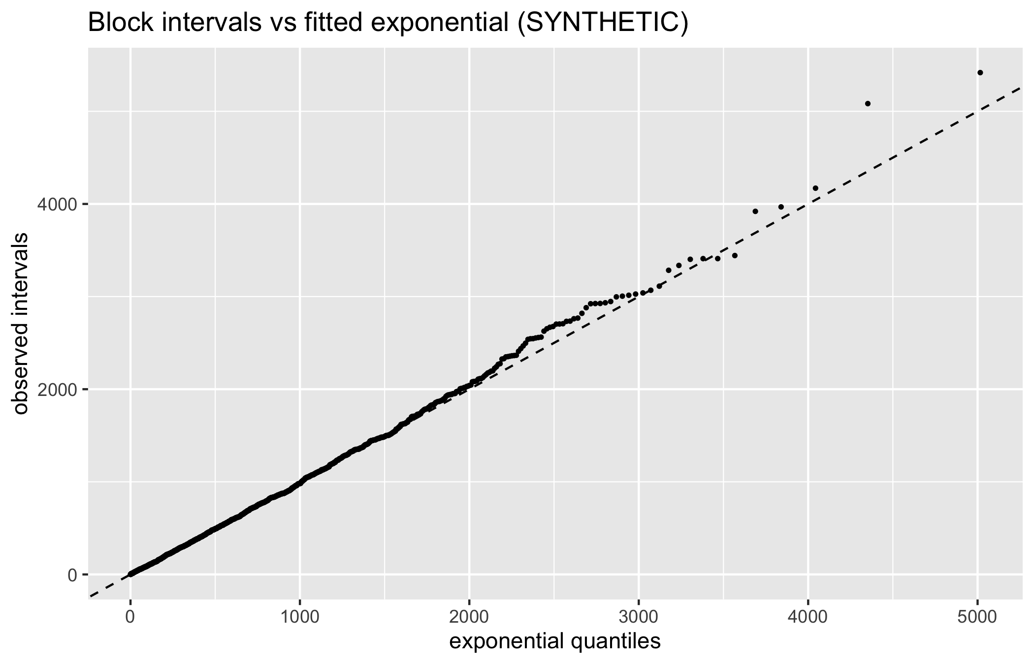
set.seed(13)# SYNTHETIC: intervals from Exp(mean 600s), the very# model under test. Swap in a real CSV to test a chain.intervals<-rexp(2016, rate =1/600)fit_rate<-1/mean(intervals)ks<-ks.test(intervals, 'pexp', rate =fit_rate)c(mean_interval =mean(intervals), fitted_rate =fit_rate, ks_p_value =ks$p.value)#> mean_interval fitted_rate ks_p_value #> 6.041721e+02 1.655158e-03 5.352700e-01ggplot(tibble::tibble( x =sort(intervals), theo =qexp(ppoints(length(intervals)), fit_rate)),aes(theo, x))+geom_point(size =0.6)+geom_abline(linetype =2)+labs(x ='exponential quantiles', y ='observed intervals', title =paste('Block intervals vs fitted','exponential (SYNTHETIC)'))
Figure 5.7: Block intervals against the fitted exponential (SYNTHETIC). On real data the interesting departures cluster around retargets and hash-rate shocks.
The QQ plot lies on the diagonal and the Kolmogorov-Smirnov test does not reject, because we drew from the model. Now we exploit the same intervals for the two estimates the chapter developed. Taking difficulty 3 as the toy analogue, the implied hash rate and the orphan rate for a five-second propagation window are read off directly.
On genuine data the science is exactly where this tidy picture breaks. Around difficulty retargets, or during hash-rate shocks such as the one the controller absorbed above, the memoryless assumption frays, the QQ plot bends away from the diagonal, and the KS test begins to reject. Reporting that boundary honestly, rather than declaring a clean fit, is the statistician’s contribution to on-chain measurement.
In conclusion, three points are to be emphasized. First, block arrivals are arrival data, and the exponential and Poisson machinery a biostatistician already owns, together with the quantile-quantile and goodness-of-fit diagnostics of survival analysis, is the correct and sufficient toolkit for on-chain timing; it should be the first instrument reached for, not a borrowed metaphor. Second, difficulty adjustment warrants reading as a discrete-time feedback controller acting on the generating rate, and questions about recovery after a hash-rate change are then answerable by its transient response rather than by folklore about difficulty always rising or by appeal to a continuous equilibrium force that does not exist. Third, the value of the statistician lies as much in stating where the memoryless model fails, through propagation delay, non-constant hash rate, and timestamp noise, as in fitting it, for those rejections, whether encountered on a chain or in a disease-surveillance stream, are where the science resides. The reader who carries these three points away has, we believe, grasped the essential argument of the chapter.
5.12 Collaborating with an LLM
An AI assistant is a capable partner for the algebra and the plotting here, and an unreliable one for the modelling judgements. It should be used with the following discipline.
Prompt. ‘Derive the orphan-rate formula for a Poisson block process with mean interval mu and propagation window Delta, and give the small-Delta approximation.’
Watch for: a confident derivation that silently assumes propagation is instantaneous, or that conflates the probability of a fork with the long-run fraction of orphaned blocks (they differ once forks can themselves fork).
Verification: re-derive from \(P(T < \Delta) = 1 - e^{-\Delta/\mu}\) independently, and confirm the \(\Delta/\mu\) limit against the simulation in the fork-rate section. The model presupposes a single competing miner within the window; state that assumption explicitly.
Prompt. ‘Write R to estimate Bitcoin hash rate from a vector of block timestamps and difficulty.’
Watch for: an estimator that omits the \(2^{32}\) (or \(16^{d}\)) work factor, that reports a point estimate with no uncertainty, or that treats raw timestamps as exact arrival times despite their known miner-set tolerance.
Verification: check the units by dimensional analysis (work per block divided by seconds per block yields hashes per second), and confirm the relative standard error scales as \(1/\sqrt{n}\) by resampling.
Prompt. ‘Explain why block times return to ten minutes after hash rate doubles.’
Watch for: an answer that credits the return to an equilibrium force acting continuously, rather than to a once-per-epoch discrete controller with a dead-time lag.
Verification: run the retarget simulation and confirm the recovery is stepwise at epoch boundaries, not smooth, and that the transient persists for up to a full epoch.
5.13 Exercises
Superposition. Two mining pools hash at rates \(r_1\) and \(r_2\). Prove that the combined block process is Poisson with rate \(p(r_1 + r_2)\) and that, given a block is found, the probability it came from pool 1 is \(r_1 / (r_1 + r_2)\), independent of the arrival time. Verify by simulation.
Geometric to exponential. Show analytically that as \(p \to 0\) with \(rp = \lambda\) held fixed, the Geometric\((p)\) attempt count, rescaled by the hash rate \(r\) into a time, converges in distribution to Exponential\((\lambda)\). Then reproduce the convergence numerically by driving mine_attempts() at increasing difficulty and overlaying the exponential limit.
Controller stability. Modify simulate_retarget() to clamp the per-epoch adjustment factor to \([1/4, 4]\), as Bitcoin does. Apply a four-fold hash-rate jump and compare the transient and any overshoot with and without the clamp. Characterise the trade-off between tracking speed and oscillation.
Fork rate versus block time. Using orphan_prob(), plot the orphan rate against mean block time for a fixed propagation window, on a log-log scale. Confirm the near-unit slope predicted by the \(\Delta/\mu\) approximation and identify where the exact expression departs from it.
Hash-rate estimator coverage. By Monte Carlo, verify that the 95 percent interval in estimate_hashrate() attains nominal coverage for \(n = 2016\), and investigate its coverage for small \(n\) (say \(n = 20\)), where the normal approximation to the exponential-mean sampling distribution is poor. Propose and test a gamma-based interval.
Model failure. Generate intervals whose rate changes partway through an epoch (a hash-rate shock), fit a single exponential, and show through the QQ plot and KS test that the pooled fit is rejected even though each segment is exponential. Discuss how this maps onto a survival analysis with an unmodelled change-point in the hazard.
5.14 Further reading
Nakamoto (2008) introduces proof-of-work and the difficulty-adjustment target; read Section 4 and the difficulty discussion as the primary source for the retarget rule.
Kraft (2016) analyses difficulty adjustment explicitly as a control problem and studies its stability, the framing this chapter adopts.
Bowden et al. (2020) is the essential empirical companion: it models Bitcoin block-arrival times and documents precisely where the homogeneous Poisson model fails, motivating non-homogeneous and doubly-stochastic refinements.
Decker & Wattenhofer (2013) measures block propagation in the real Bitcoin network and connects propagation delay to the fork rate, grounding the orphan-rate calculation in observed data.
Goffard (2023), the BLOCKASTICS course materials, are the closest existing statistics-course precedent, presenting blockchain as a subject for a probability and statistics curriculum; they are the natural next text for a reader who wants this chapter’s viewpoint extended.
Narayanan et al. (2016) remains the rigorous reference textbook; its treatment of mining and difficulty complements the process-oriented account given here.
Bowden, R., Keeler, H. P., Krzesinski, A. E., & Taylor, P. G. (2020). Modeling and analysis of block arrival times in the Bitcoin blockchain. Stochastic Models, 36(4), 602–637. https://doi.org/10.1080/15326349.2020.1786404
Goffard, P.-O. (2023). BLOCKASTICS: Stochastic models for blockchain analysis (course materials). University course, Lyon 1 / Strasbourg. https://pierre-olivier.goffard.me/BLOCKASTICS/
Kraft, D. (2016). Difficulty control for blockchain-based consensus systems. Peer-to-Peer Networking and Applications, 9, 397–413. https://doi.org/10.1007/s12083-015-0347-x
Nakamoto, S. (2008). Bitcoin: A peer-to-peer electronic cash system. Self-published whitepaper. https://bitcoin.org/bitcoin.pdf
Narayanan, A., Bonneau, J., Felten, E. W., Miller, A., & Goldfeder, S. (2016). Bitcoin and cryptocurrency technologies: A comprehensive introduction. Princeton University Press. https://bitcoinbook.cs.princeton.edu/