The race between the honest chain and an attacker chain can be characterized as a Binomial Random Walk.
Satoshi Nakamoto, Bitcoin: A Peer-to-Peer Electronic Cash System (2008)
4.1 Learning objectives
By the end of this chapter the reader should be able to:
State the proof-of-work puzzle as a Bernoulli search over nonces and explain why it is progress-free (memoryless).
Describe Nakamoto consensus, the longest-chain (most-work) rule, and how cost substitutes for identity to resist Sybil attacks.
State the three Bitcoin Backbone properties (common prefix, chain quality, chain growth) precisely and say what each guarantees.
Derive the simple gambler’s-ruin bound \((q/p)^z\) for a double-spend and explain how Satoshi’s Poisson mixture refines it.
Compute an attacker-success probability, verify the six-confirmations claim, and cross-check the closed form by simulation.
Treat confirmation depth as a tail-probability threshold, the same decision as choosing a critical value or a group-sequential stopping boundary.
4.2 Orientation
We begin with a data problem. Consider a consortium of hospitals running a multi-site clinical trial. Enrolment, randomisation, and outcome events are appended to a shared, append-only log that no single institution owns, and a regulator will audit that log after the fact. We shall refer to this arrangement throughout as the trial ledger. Suppose an outcome event, the death of a subject, say, or a confirmed endpoint, is appended at one site. Here is the question that governs everything downstream: how long must the other sites wait before they may treat that event as settled, so that an interim analysis, or a report to the data and safety monitoring board, may rely upon it? Act too soon and the record may yet be revised beneath the analysis; wait too long and the monitoring that safeguards the trial’s subjects is delayed.
The previous two chapters assembled the parts. Chapter 2 posed open-membership Byzantine agreement as the problem, and Chapter 3 supplied the hash function that behaves as a random oracle. This chapter puts them together into the mechanism that made Bitcoin work, and although digital cash is the historical setting in which that mechanism was born, our interest here is in what it offers the trial ledger. The vocabulary is one the reader already owns. The proof-of-work puzzle is a sequence of independent Bernoulli trials, that is, repeated yes-or-no experiments, each with a minuscule success probability. The security of a confirmed record is the tail of a biased random walk. The choice of how long to wait before treating a record as settled is the choice of a critical value: a threshold on a quantified error probability.
The single most important reframing in the chapter is this. A blockchain does not give certainty that a record is permanent. It gives a probability that the record will be reversed, and that probability decays geometrically in the number of blocks mined on top of it. ‘Finality’ is therefore not a binary state the ledger enters. It is a confidence statement, and the reader who has ever chosen a significance level, or set a stopping boundary for a group-sequential trial, already knows how to reason about it.
We shall build every claim twice: once as a piece of mathematics, and once as runnable R that the reader may re-execute. The attacker-success calculation reproduced here is that of Satoshi Nakamoto, the pseudonymous author of the 2008 Bitcoin whitepaper, given in its Section 11 (Nakamoto, 2008), and we verify the six-confirmations claim rather than repeat it on faith.
Before proceeding we fix the terminology on which the remainder of the chapter depends, so that the reader need not carry these terms as mysteries.
NoteThe vocabulary of this chapter
Proof-of-work. A scheme in which appending a block requires solving a computational puzzle that is costly to perform but cheap to check, so that influence over the ledger is bought with computation rather than with identity.
Nonce. A number placed in a block header and varied by the miner in search of a header whose hash meets the target. It is the one field the miner is free to change at will.
Target and difficulty. The target is the threshold a block hash must fall below to be valid; the difficulty is the reciprocal measure of how demanding that threshold is. A smaller target means a higher difficulty and more expected work per block.
Nakamoto consensus. The procedure, introduced with Bitcoin, by which open and mutually distrusting parties agree on one history: they extend and accept the chain carrying the most accumulated proof-of-work.
Longest-chain (heaviest-chain) rule. The fork-choice component of Nakamoto consensus: honest nodes treat the chain with the greatest total work as authoritative, which reduces to the longest chain when difficulty is held constant.
Fork and orphan block. A fork is a temporary split in which two valid blocks extend the same parent. When one branch is abandoned, the discarded block is termed an orphan, and the transactions it held return to the pending pool.
Double-spend. The canonical attack, in which a party spends a record, waits for it to be accepted, and then publishes a competing chain that erases it, thereby reversing a transaction already treated as settled.
Probabilistic finality and confirmation depth. A confirmed record is never permanent with certainty; the probability of its reversal merely shrinks as further blocks accumulate above it. The confirmation depth is the number of such blocks, written \(z\), at which one agrees to treat the record as settled.
4.3 The statistician’s contribution
Three judgements in this chapter fall to the analyst, and no protocol automates them.
1. Finality is a confidence statement, not a fact. The protocol emits a reversal probability; a human decides how small it must be before acting. That is a critical value chosen against a quantified tail risk, and setting it well requires knowing the cost of a wrong decision, which the chain cannot know on our behalf. A merchant selling coffee, a clearing house settling a bond, and a monitoring board acting on an interim endpoint should not use the same depth.
2. The model’s assumptions are where the real risk resides. Satoshi’s bound assumes a fixed attacker hash share \(q\), honest blocks arriving as a Poisson process, and no network partition. Each assumption can fail: hash-rate can be rented in bursts, propagation delay creates natural forks, and a sufficiently resourced adversary changes \(q\) mid-attack. Naming which assumption a given deployment violates is the analyst’s job, not the whitepaper’s.
3. ‘Immutable’ is a claim to be demoted. The correct statement is ‘exponentially expensive to revise, with the exponent set by depth and the base set by the honest majority margin’. Reporting the number, not the adjective, is the contribution.
4.4 The proof-of-work puzzle
4.4.1 The puzzle as a Bernoulli search
A block header commits to the previous block’s hash, a Merkle root of the transactions (a hash-based summary that commits to every transaction in the block), a timestamp, and a nonce. To mine a block a miner searches for a nonce such that the header hash, read as a 256-bit integer, falls below a target \(T\):
\[
H(\text{header}) < T .
\]
Because \(H\) behaves as a random oracle, an idealised function whose every output is, in effect, an independent uniform draw (Chapter 3), each distinct nonce yields an output that is, for all practical purposes, uniform on \(\{0, 1, \dots, 2^{256}-1\}\). A single attempt therefore succeeds with probability
\[
p = \frac{T}{2^{256}} ,
\]
independently across nonces. Mining is a sequence of i.i.d. Bernoulli\((p)\) trials with \(p\) extremely small.
It is often more intuitive to state the puzzle in leading zero bits. If the target requires the top \(d\) bits of the hash to be zero, then
\[
p = 2^{-d} ,
\]
and the expected number of attempts to find a block is \(1/p = 2^{d}\). Each additional required zero bit halves the success probability and doubles the expected work. Stated in hexadecimal digits, each leading hex zero divides the valid target set by 16, a fact we will measure directly in Chapter 5.
4.4.2 Progress-free means memoryless
The property that makes proof-of-work a fair lottery rather than a race is that it is progress-free. A miner who has failed a million times is in exactly the same position as a miner who just started: the next attempt still succeeds with probability \(p\). There is no partial credit, no accumulated progress toward the solution. Formally, the number of attempts \(N\) until the first success is geometric,
and the geometric distribution is the unique memoryless distribution on the positive integers:
\[
\Pr(N > m + n \mid N > m) = \Pr(N > n) .
\]
Memorylessness has a consequence the reader will recognise. When many independent miners each run their own tiny-\(p\) Bernoulli search in parallel, the time until some miner succeeds is, in the continuous limit, exponential, and the stream of blocks is a Poisson process (the standard model for events that arrive independently at a steady average rate). That is the entire statistical foundation of the next chapter, so we flag it here and develop it in Chapter 5.
Progress-freedom is also what makes hash-power the sole determinant of success. One cannot be clever about finding a nonce; one can only attempt more of them per second. Mining reduces one resource, computation, to one number, and that reduction is what lets cost stand in for identity.
NoteCheck your understanding: doubling the difficulty
A chain currently requires \(d\) leading zero bits, so a block takes an expected \(2^{d}\) hash attempts. The difficulty is raised to require \(d+3\) zero bits. By what factor does the expected number of attempts per block change, and does a miner who has already tried \(2^{d}\) nonces at the new difficulty have any advantage on the next attempt?
The expected attempts rise by a factor of \(2^{3} = 8\), since \(\mathbb{E}[N] = 2^{d+3} =
8 \cdot 2^{d}\). The miner has no advantage: the search is progress-free, so having tried \(2^{d}\) nonces leaves the success probability of the next attempt at exactly \(2^{-(d+3)}\), unchanged. Past failures carry no information about future success. This is the memoryless property, and it is why a large miner’s advantage is strictly proportional to hash-rate, with no economies of scale in the search itself.
4.5 Nakamoto consensus
4.5.1 The longest-chain rule
Proof-of-work resolves the question of which party may append the next block. Nakamoto consensus resolves the question of which chain the parties agree upon. The rule is simple to state: honest nodes always extend the chain with the most accumulated proof-of-work, and treat that chain as the truth. In the common case where difficulty is constant, most-work reduces to longest, so the mechanism is usually called the longest-chain rule.
The rule is a decentralised tie-break. When two miners find a block at nearly the same time, the network temporarily holds two competing chains of equal length. The tie resolves when the next block extends one of them; that chain now has more work, honest nodes switch to it, and the orphaned block’s transactions return to the pool. No vote is taken and no coordinator is consulted. The heaviest chain wins by construction.
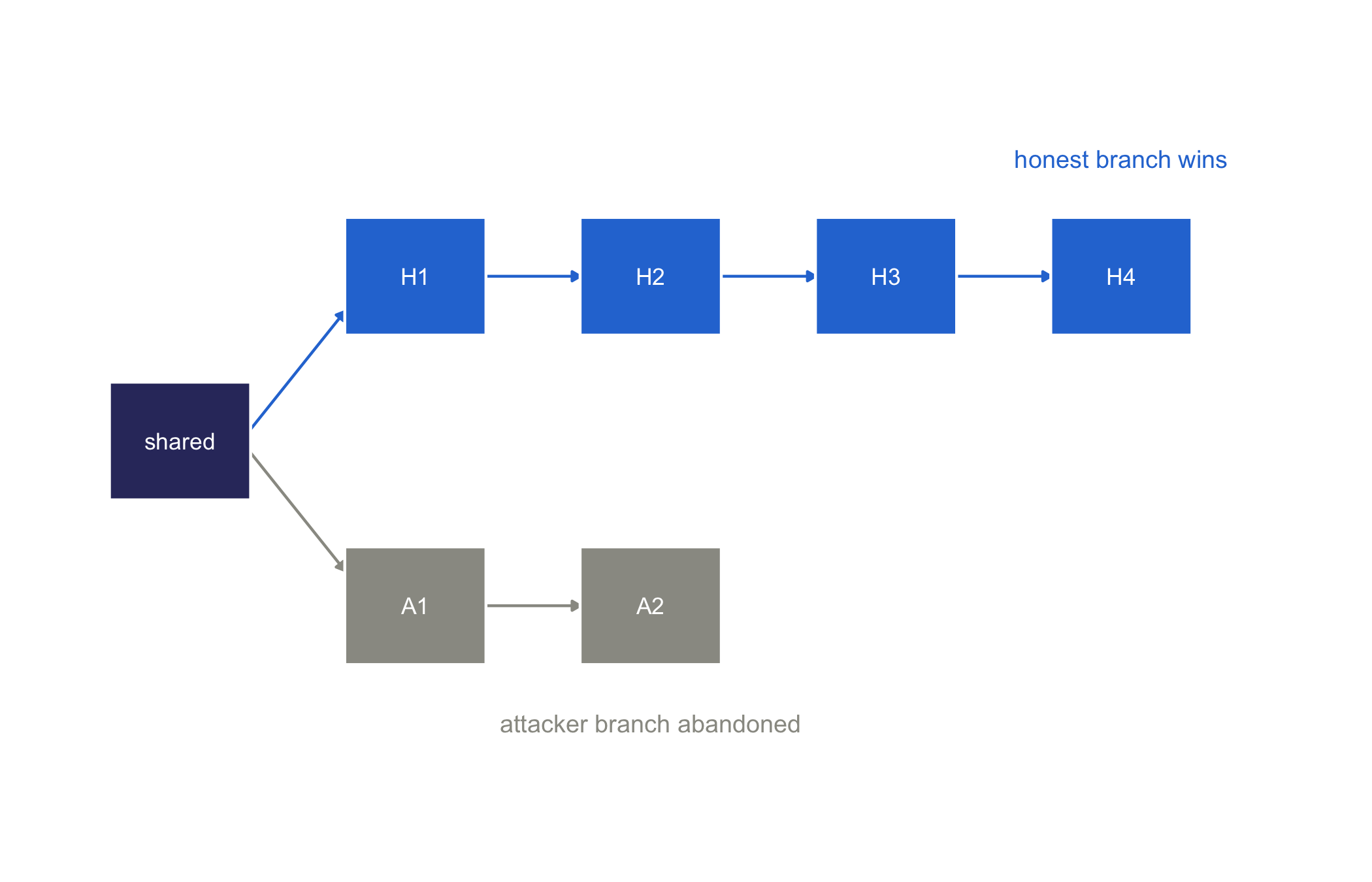
We can picture the tie-break directly. Figure 4.1 shows two branches leaving a shared block: the honest branch pulls ahead, and the attacker branch, once it falls behind, is abandoned.
Figure 4.1: A fork resolves by accumulated work: honest nodes follow the heavier branch, so the honest chain that pulls ahead wins and the attacker branch that falls behind is abandoned.
4.5.2 Cost substitutes for identity
The reason this survives an open-membership setting is that appending a block costs real computation, so votes are weighted by hash-power rather than by identity. In a classical Byzantine agreement protocol (Chapter 2) an adversary who can forge identities can manufacture a majority: the Sybil attack (Douceur, 2002). Nakamoto consensus makes identities free but makes influence expensive. Creating a thousand fake nodes confers no advantage, because each block still requires the same expected \(1/p\) hash attempts. To outweigh the honest network an attacker must out-compute it, which is the content of the phrase ‘one CPU, one vote’ in the whitepaper, correctly read as ‘one unit of hash-power, one unit of vote’.
This is the pivotal design move. The Sybil problem is not solved by authenticating participants; it is dissolved by making the scarce resource external and physical. Proof-of-work is, in the language of Dwork & Naor (1993) who first proposed pricing via processing, a cost function that gates participation.
4.5.3 Probabilistic finality
Because an attacker with a minority of hash-power can still, by chance, find several blocks in a row, no transaction is ever absolutely final. What the longest-chain rule delivers is that the probability of reversing a transaction buried under \(z\) subsequent blocks decays geometrically in \(z\). Finality is asymptotic, approached but never reached.
Here the public-health reader has a ready analogy. In group-sequential monitoring of a trial we do not wait for the study to end before acting; we examine the accumulating data at interim looks and act when the evidence crosses a stopping boundary chosen to control the overall error probability. Waiting for confirmations is the same shape of decision. Each new block is a further look at the ledger, and we treat a record as settled once the reversal probability has fallen below a boundary we have set in advance. The analogy is honest, but it has a limit, and we should mark it plainly. In group-sequential monitoring the uncertainty is sampling error, and the data, once recorded, do not conspire against us. In the ledger the uncertainty is adversarial: a reorganisation is not the luck of the draw but the product of an attacker spending hash-power to rewrite history. The tail we compute is therefore a bound against a strategic opponent, not a sampling distribution, and that distinction warrants a more conservative boundary than sampling error alone would demand.
This is the deepest contrast with the classical Byzantine-fault-tolerant protocols studied in Chapter 2 and revisited for proof-of-stake in Chapter 10. A protocol such as PBFT, or Practical Byzantine Fault Tolerance, the protocol of Castro and Liskov (Castro & Liskov, 1999), delivers deterministic finality within a known number of rounds, at the cost of a fixed, known validator set. Nakamoto consensus buys open membership at the price of finality that is only ever probabilistic. Neither is strictly better; they price the same guarantee in different currencies, and knowing which one is buying is the point.
ImportantThe sceptic’s reflex
The reader will encounter the claim that a blockchain is ‘immutable’ and that confirmed transactions are ‘permanent’. The tier should be named. ‘Immutable’ is delivered in the cadence of a protocol fact, but the protocol fact is weaker and more precise: a confirmed transaction is exponentially expensive to revise, with a reversal probability that is small but never zero and that depends on the attacker’s hash share. ‘Immutable’ should be demoted to ‘exponentially expensive to revise, and here is the exponent’. The adjective hides exactly the quantity a statistician is equipped to report.
4.6 The Bitcoin Backbone
Satoshi’s whitepaper argued security by a single tail-probability calculation. A decade of formal work, initiated by the Bitcoin Backbone analysis of Garay, Kiayias, and Leonardos (Garay et al., 2015), which recast Nakamoto’s informal security argument as a set of provable guarantees, and extended to the asynchronous setting by 1, distilled the protocol into three properties that hold with overwhelming probability provided the honest parties control a sufficient majority of hash-power. The properties are stated over the chains held by honest parties as the protocol runs.
Common prefix. For any two honest parties at any two times, the shorter chain, after removing its last \(k\) blocks, is a prefix of the longer chain, except with probability dropping exponentially in \(k\). In words: honest parties agree on all but the most recent few blocks. This is precisely what licenses ‘wait \(z\) confirmations’: the common-prefix parameter \(k\) is the confirmation depth, and the exponential drop is the reversal probability. Common prefix is the formal home of probabilistic finality.
Chain quality. In any sufficiently long window of an honest party’s chain, the fraction of blocks contributed by honest parties is bounded below (roughly by the honest hash share, degraded by an adversarial factor). In words: the adversary cannot monopolise the ledger’s content. Chain quality guarantees that honest transactions actually get included, not merely that parties agree on some ordering. Without it a majority-but-not-total attacker could agree with everyone while censoring chosen transactions.
Chain growth. The honest parties’ chains grow by at least a guaranteed number of blocks in any sufficiently long window. In words: the ledger makes progress, it does not stall. Chain growth is what lets us assume that waiting real time produces confirmations at a predictable rate, which is the premise of every latency calculation in Chapter 5.
The three properties are complementary. Common prefix is safety (agreement), chain growth is liveness (progress), and chain quality is a fairness or censorship-resistance guarantee sitting between them. Stated compactly: common prefix says honest parties agree, chain growth says they keep moving, chain quality says the adversary cannot fill the chain with its own blocks. All three degrade gracefully rather than failing catastrophically as the adversary approaches the honest-majority threshold.
Table 4.1 collects the three properties beside what each guarantees and how we read it for the trial ledger.
Table 4.1: The three Bitcoin Backbone properties, what each guarantees, and how the trial ledger reads it
Property
Informal statement
What it guarantees
Trial-ledger reading
Common prefix
Honest parties agree on all but the last few blocks
Safety: no reorganisation below depth \(k\)
The \(z\) in ‘wait \(z\) confirmations’ is this \(k\)
Chain quality
The adversary cannot monopolise the block content
Censorship resistance: honest events get in
A settled outcome event cannot be quietly excluded
Chain growth
The chain gains blocks at a guaranteed rate
Liveness: the ledger does not stall
Confirmations accrue in predictable real time
4.6.1 GHOST, an alternative fork-choice
The longest-chain rule discards the work in orphaned blocks. When block propagation is slow relative to the block interval, forks are frequent, orphaned work is large, and security suffers because the effective honest hash-power is fragmented. The GHOST rule (Greedy Heaviest Observed Subtree) of Sompolinsky and Zohar (Sompolinsky & Zohar, 2015) changes the fork-choice: rather than following the longest chain, a node at each fork follows the subtree containing the most total work, counting orphaned blocks toward the weight of their branch. This lets a chain tolerate faster block times without the security loss that naive longest-chain would suffer, and a variant of it informed Ethereum’s early fork-choice. The point for our purposes is that longest-chain is one fork-choice rule among several, each with a different tradeoff between block interval, orphan rate, and security, and each analysable by the same probabilistic tools.
4.7 Double-spend as gambler’s ruin
4.7.1 The random-walk model
We now come to the chapter’s mathematical core, and we shall frame it from the outset as the computation of the very error probability the trial ledger requires. The canonical attack on Nakamoto consensus is the double-spend. An attacker pays a merchant, waits for the transaction to be buried under \(z\) confirmations, takes delivery of the goods, and then attempts to publish a longer private chain that omits the payment, reversing it. The attack succeeds if and only if the attacker’s private chain overtakes the honest chain. The same adversary threatens the trial ledger: a site that wishes to un-record a settled outcome event must, by exactly this mechanism, outpace the honest sites, and the probability that it succeeds is the probability that our ‘settled’ verdict was premature.
Model the race by the lead of the honest chain over the attacker. Let the attacker command a fraction \(q\) of total hash-power and the honest network \(p = 1 - q\), with \(q < p\). Each new block is honest with probability \(p\) and attacker’s with probability \(q\). The gap between the chains is a random walk that steps \(+1\) (honest extends its lead) with probability \(p\) and \(-1\) (attacker closes the gap) with probability \(q\). The attacker wins if this walk ever reaches zero starting from a lead of \(z\).
This is the classical gambler’s ruin, the problem of a bettor with finite capital playing against a richer adversary until one side is exhausted, and its solution is well known. For a walk biased away from the origin (\(q < p\)), the probability of ever reaching zero starting from distance \(z\) is
\[
\Pr(\text{catch up from } z)
= \left( \frac{q}{p} \right)^{z} .
\]
The derivation is the standard one. Let \(a_z\) be the catch-up probability from a gap of \(z\). First-step analysis gives \(a_z = q\,a_{z-1} +
p\,a_{z+1}\) with \(a_0 = 1\), whose bounded solution for \(q < p\) is \(a_z = (q/p)^{z}\). The security of \(z\) confirmations, in this simplest model, is that reversal probability falls geometrically with ratio \(q/p < 1\). If the attacker holds ten percent of hash-power, \(q/p = 1/9\), and each confirmation cuts the reversal odds by a factor of nine.
4.7.2 Satoshi’s Poisson refinement
The simple bound \((q/p)^{z}\) is pessimistic in one respect and optimistic in another, and Satoshi’s Section 11 calculation corrects it. The subtlety is that during the time the honest network builds its \(z\) confirmations, the attacker is not idle: it is mining its private chain in parallel. So at the moment the merchant accepts, the attacker has already made some private progress.
Satoshi models this as follows. While the honest network finds \(z\) blocks, the number of blocks the attacker finds is Poisson with mean
\[
\lambda = z \, \frac{q}{p} ,
\]
since the attacker’s blocks arrive at rate \(q/p\) relative to the honest network’s. Condition on the attacker having found \(k\) private blocks. If \(k \ge z\) the attacker is already ahead and succeeds with probability one. If \(k < z\) the attacker is behind by \(z - k\) and must close that gap, which by gambler’s ruin happens with probability \((q/p)^{z-k}\). Mixing over the Poisson distribution of \(k\),
This is the formula we now evaluate. It refines the crude \((q/p)^z\) by accounting for the attacker’s head start, and it is precisely the reversal probability the trial ledger needs: the chance that a record treated as settled at depth \(z\) is later undone. But how deep is deep enough? The question has no answer in the abstract, for the depth that suffices depends on the attacker share we are willing to assume and the tolerance we are willing to accept. We begin with the case Satoshi treats, an attacker holding ten percent of hash-power who is watched to a depth of six.
p_attack<-function(q, z){p<-1-qlambda<-z*(q/p)k<-0:z1-sum(dpois(k, lambda)*(1-(q/p)^(z-k)))}# Satoshi's claim: q = 0.10, z = 6 gives well under 0.1 percent.p_attack(0.10, 6)#> [1] 0.0002428027
The value is well below one in a thousand, confirming the whitepaper’s assertion that six confirmations suffice against an attacker with ten percent of hash-power. This is the origin of the folk rule ‘wait for six confirmations’: it is not an arbitrary constant but the depth at which the Section 11 tail probability drops below a tolerance a merchant, or a monitoring board, is willing to accept. A different tolerance implies a different depth.
It is worth seeing the whole tail at once. Table 4.2 tabulates the reversal probability across depths and attacker shares, the table a merchant or a monitoring board reads down a column to the depth at which the probability first falls below its tolerance.
library(knitr)qs<-c(0.05, 0.10, 0.25, 0.40)zs<-0:12tab<-sapply(qs, function(q)sapply(zs, function(z)p_attack(q, z)))tab_df<-data.frame(z =zs, formatC(tab, format ='e', digits =2), check.names =FALSE)names(tab_df)<-c('z', paste0('q = ', formatC(qs, format ='f', digits =2)))knitr::kable(tab_df, align ='r', caption ='Reversal probability P(success) by confirmation depth z (rows) and attacker hash share q (columns), from the Section 11 formula. Reading down a column shows the geometric decay for a fixed attacker; comparing columns shows how the depth needed for a target tolerance climbs as q grows.')
Table 4.2: Reversal probability P(success) by confirmation depth z (rows) and attacker hash share q (columns), from the Section 11 formula. Reading down a column shows the geometric decay for a fixed attacker; comparing columns shows how the depth needed for a target tolerance climbs as q grows.
z
q = 0.05
q = 0.10
q = 0.25
q = 0.40
0
1.00e+00
1.00e+00
1.00e+00
1.00e+00
1
1.01e-01
2.05e-01
5.22e-01
8.29e-01
2
1.26e-02
5.10e-02
3.15e-01
7.36e-01
3
1.64e-03
1.32e-02
1.96e-01
6.64e-01
4
2.16e-04
3.46e-03
1.24e-01
6.03e-01
5
2.87e-05
9.14e-04
7.84e-02
5.51e-01
6
3.84e-06
2.43e-04
4.99e-02
5.04e-01
7
5.14e-07
6.47e-05
3.19e-02
4.62e-01
8
6.90e-08
1.73e-05
2.05e-02
4.25e-01
9
9.29e-09
4.63e-06
1.31e-02
3.91e-01
10
1.25e-09
1.24e-06
8.45e-03
3.60e-01
11
1.69e-10
3.33e-07
5.44e-03
3.32e-01
12
2.27e-11
8.95e-08
3.50e-03
3.06e-01
4.7.3 The family of attack curves
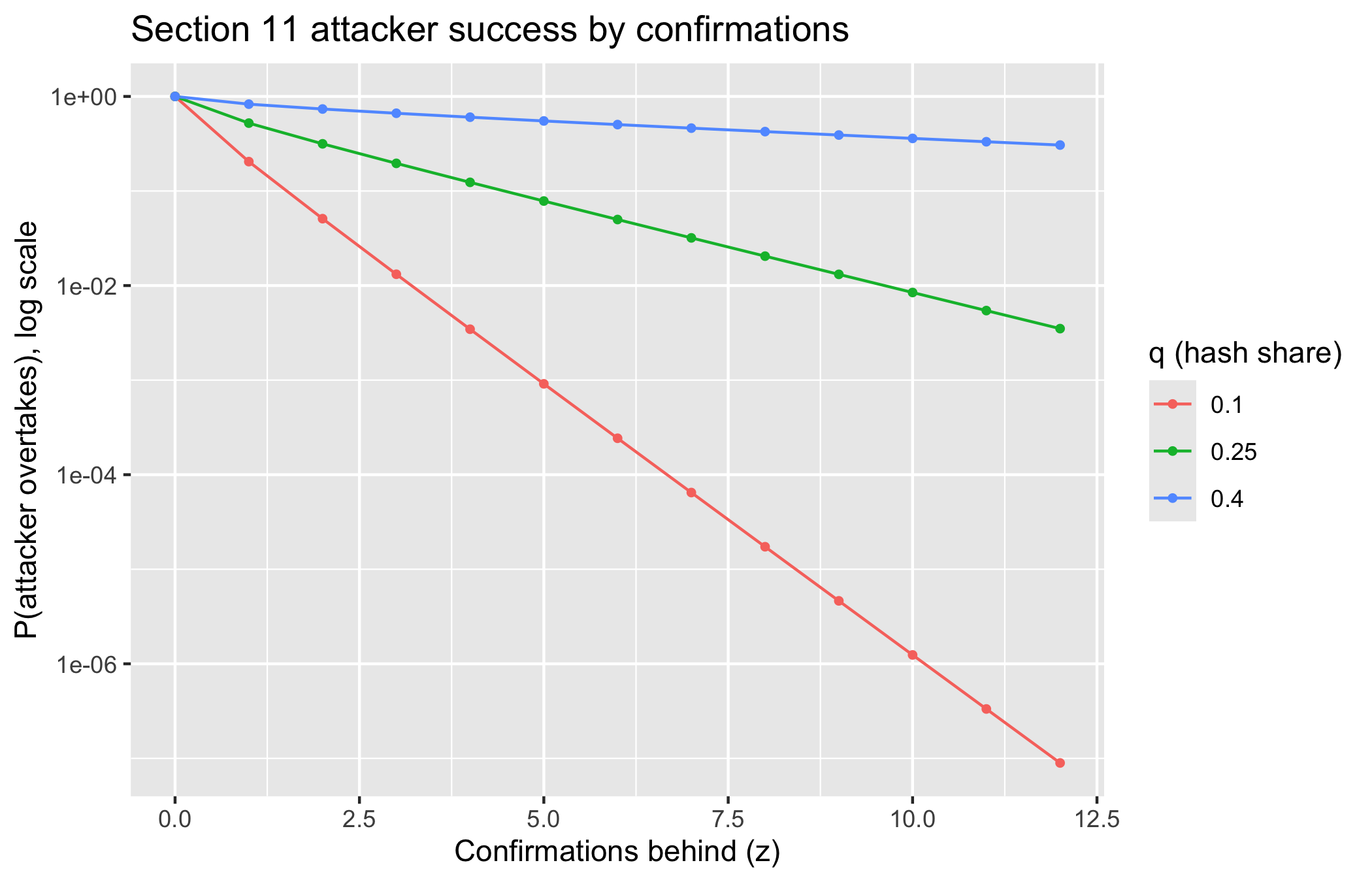
Plotting the attack probability against confirmation depth for several attacker shares makes the geometric decay, and its sensitivity to \(q\), visible at once.
Figure 4.2: Attacker success probability by confirmation depth z, for hash shares q in {0.10, 0.25, 0.40}, on a log scale. Deeper confirmations buy exponentially more security, but the slope flattens as q approaches one half.
Read Figure 4.2 as a statistician reads a power curve. For \(q = 0.10\) the reversal probability falls steeply, and six confirmations already place it out of reach. For \(q = 0.40\) the curve is nearly flat: an attacker with forty percent of hash-power is so close to parity that no realistic confirmation depth secures the transaction, because the random walk’s drift away from zero is weak. The confirmation depth that buys a target security level is a function of the attacker share we are willing to assume, and assuming \(q\) is a modelling decision, not a protocol output.
4.7.4 Cross-checking the closed form
A closed-form probability should always be checked against a simulation of the same model, if only to catch transcription errors. We draw the attacker’s private block count as Poisson, resolve the residual gap by the gambler’s-ruin ratio, and compare.
The two columns agree to simulation noise. Note the honest epistemic claim: agreement validates the transcription of the model into code, not the model itself. The model is Satoshi’s, and its assumptions (fixed \(q\), Poisson honest blocks, no partition) are the things a deployment can violate. A simulation cannot vindicate an assumption it also makes.
NoteCheck your understanding: choosing a depth is choosing a critical value
A merchant will accept a transaction once the reversal probability falls below a tolerance \(\alpha\). Explain in what precise sense choosing the confirmation depth \(z\) is the same kind of decision as choosing a critical value in a hypothesis test, and what plays the role of the ‘cost of a Type I error’.
The reversal probability \(\Pr(\text{success})\) is a monotone decreasing function of \(z\). Choosing the smallest \(z\) with \(\Pr(\text{success}) \le \alpha\) is exactly choosing a rejection threshold so that a tail probability sits below a preset level, the same operation as picking a critical value so that \(\Pr(\text{Type I error}) \le \alpha\). The tail here is the tail of the biased random walk rather than of a null sampling distribution, but the logic is identical: fix the tolerable error probability, then read off the threshold. The ‘cost of a wrong decision’ is the value of the goods released against an unconfirmed payment; higher stakes justify a smaller \(\alpha\) and hence a deeper \(z\), just as a costlier false positive justifies a stricter significance level. The chain supplies the tail; the human supplies \(\alpha\).
4.7.5 Setting the depth in practice
We may now return to the question with which the chapter opened. How many confirmations should elapse before the trial ledger treats an appended outcome event as settled, so that an interim analysis or a report to the monitoring board may rely upon it? The machinery of the preceding sections answers it directly. The reversal probability is \(\Pr(\text{success})\) as a function of the assumed attacker share \(q\) and the depth \(z\), and the required depth is the smallest \(z\) at which that probability falls below the tolerance we are prepared to accept.
To illustrate, consider the trial ledger with an assumed adversary share \(q = 0.10\) and ten-minute blocks. A monitoring board content with a reversal probability below one in a thousand may act at a depth of six, which by p_attack(0.10, 6) is roughly one chance in four thousand and corresponds to about an hour of waiting. A board that judges the stakes higher, and demands one in a million, must wait to a depth of eleven, since \(\Pr(\text{success})\) first crosses \(10^{-6}\) between \(z = 10\) and \(z = 11\), which is under two hours. The extra security is bought with roughly fifty additional minutes of latency, and whether that trade is worth making is a judgement about the trial, not about the chain.
The tradeoff is exactly the latency-versus-risk tradeoff of the double-spend calculation. Acting on a shallow confirmation is fast but exposes the workflow to a reversal: if the block is later orphaned, the outcome event it recorded is un-recorded, and any interim decision taken in reliance on it, an early-stopping recommendation, say, rests on a record that no longer exists. The same logic governs a vaccine cold-chain provenance system, our secondary example, in which each custody hand-off of a refrigerated consignment is anchored to the chain: a premature reliance on a shallow confirmation risks certifying a hand-off that is subsequently undone. Waiting for a deep confirmation is safe but slow, and in either setting the latency itself carries a cost. The decision is a threshold on a quantified reversal probability, and it should be set by the consequence of a reversal, not by a default.
Here candour is owed, and we state the limit plainly. For most health-data integrity problems the parties share a regulator or a sponsor who can serve as a custodian, and a well-governed database with a cryptographic audit log delivers tamper-evidence without any of this probabilistic-finality machinery, as Chapter 1 argued. On the one hand the confirmation-depth calculation is the right tool when the log must be trust-minimised across parties with no common authority; on the other, when a common authority does exist, the calculation is machinery in search of a problem. The analyst’s first contribution is therefore not to compute the depth but to ask whether the condition that makes the depth meaningful actually holds.
4.8 Worked example: a tamper-evident toy chain
To make the linkage concrete we build a small proof-of-work chain from scratch, then demonstrate that altering a buried block is detectable. To fix ideas, let each block hold a batch of trial events, a day’s enrolments, randomisations, and outcome records from one site, so that the data field stands for that batch. The function validate_chain is then the regulator’s audit: months after the fact, the regulator recomputes every hash and checks that the recorded history is internally consistent and carries the required proof-of-work. This is the mechanism behind ‘tamper-evident’ stated as running code rather than as an adjective. The data here are SYNTHETIC, standing in for the event batches only as the labels ‘block-1’ through ‘block-6’.
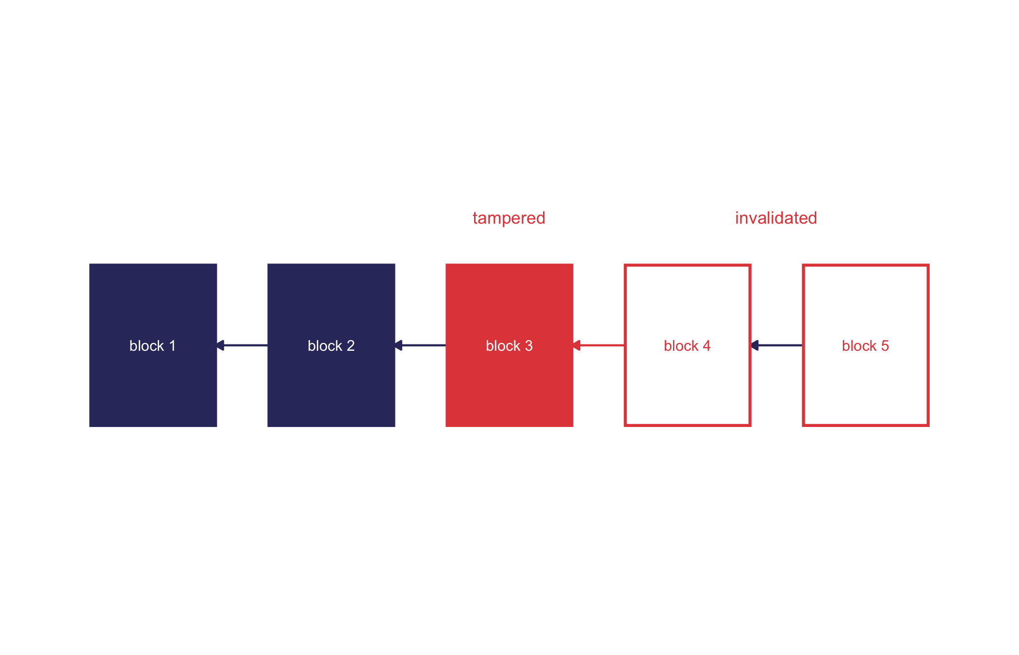
The original six-block chain validates: the regulator’s audit passes. Altering the data in block 3, as if a site had quietly revised a day’s outcome records after the fact, breaks validation for two independent reasons, both of which validate_chain checks. The recomputed hash of block 3 no longer matches its stored hash, and even had the attacker recomputed that hash, it would no longer begin with the required zero digits, nor would it match the prev_hash recorded in block 4. To repair the chain the attacker would have to re-mine block 3 and every block after it, each at full proof-of-work cost. This is the microcosm of the double-spend analysis, and the point for the trial ledger is the same one seen from the auditor’s side: a buried record cannot be revised without redoing all the work stacked upon it, and the deeper the record, the more work required. That is the gambler’s-ruin bound once more, read from the attacker’s side of the ledger.
Figure 4.3 renders the cascade the audit detects: the tamper at block 3, and the prev-hash links above it that no longer close.
Figure 4.3: Each block commits to its predecessor by a prev-hash pointer, so tampering with block 3 breaks the links above it: block 3 no longer matches the pointer carried by block 4, and the invalidation cascades to block 5.
4.9 Collaborating with an LLM
An AI assistant is useful for this material and also a frequent source of confidently stated errors. We consider three patterns, each as a Prompt, a Watch-for, and a Verification.
Prompt. ‘Derive the probability that a proof-of-work double-spend attacker with hash share q overtakes the honest chain from z blocks behind, and give the simple gambler’s-ruin bound.’
Watch for. Assistants frequently return the crude \((q/p)^z\) bound and present it as the full answer, silently dropping Satoshi’s Poisson correction for the attacker’s head start. They also sometimes invert \(q\) and \(p\), giving a bound greater than one.
Verification. Check the boundary cases by hand: the bound must equal one at \(z = 0\) and must lie in \([0, 1]\) for all \(q < p\). Compare the closed form against the mc_attack simulation above; they must agree to simulation noise.
Prompt. ‘State the three Bitcoin Backbone properties and what each guarantees.’
Watch for. Conflation of common prefix (a safety property) with chain quality (a censorship-resistance property), and omission of the honest-majority precondition under which all three hold. Some assistants invent a fourth property or attribute the framework to the wrong paper.
Verification. Map each stated property to safety, liveness, or fairness and confirm the three roles are covered exactly once. Check the attribution against Garay et al. (2015) and the asynchronous extension against
Prompt. ‘Write R to compute the six-confirmations reversal probability and plot it against depth.’
Watch for. Off-by-one errors in the Poisson sum’s upper limit, use of = for assignment or the %>% pipe against house style, and code that silently assumes \(q < p\) without flagging that the formula is invalid for \(q \ge 0.5\).
Verification. Re-run the code and reproduce p_attack(0.10, 6) below one in a thousand. Confirm the function is monotone decreasing in \(z\) and that it returns 1 at \(z = 0\).
4.10 Conclusion
In conclusion, three points are to be emphasized. First, finality on a proof-of-work ledger is a confidence statement rather than a fact, and the confirmation depth is a critical value chosen against a quantified reversal probability, the same kind of decision as setting a significance level or a stopping boundary in group-sequential monitoring; for the trial ledger, the depth at which an outcome event may be treated as settled is ours to set by the consequence of a reversal, and no protocol sets it on our behalf. Second, the gambler’s-ruin analysis, refined by Satoshi’s Poisson correction for the attacker’s head start, supplies the number, and we have verified the folk ‘six confirmations’ claim against both the closed form and a simulation rather than repeating it on faith. Third, the machinery earns its place only where the log must be trust-minimised across parties with no common authority; where a regulator or sponsor can serve as a custodian, a well-governed database with a cryptographic audit log is the more honest choice, and saying so is itself part of the analyst’s contribution.
4.11 Exercises
Leading zeros and expected work. A chain targets a hash below \(T = 2^{256 - d}\). Derive the per-attempt success probability and the expected number of attempts per block as functions of \(d\). Show that adding one required hexadecimal zero (four bits) multiplies the expected work by sixteen, and connect this to the memoryless property.
Derive the gambler’s-ruin bound. Starting from the first-step relation \(a_z = q\,a_{z-1}
+ p\,a_{z+1}\) with \(a_0 = 1\), solve for the bounded catch-up probability when \(q < p\) and obtain \(a_z = (q/p)^z\). Explain why the solution is unbounded, hence rejected, when \(q > p\), and what that says about a majority attacker.
Verify six confirmations across shares. Using p_attack, tabulate the smallest confirmation depth \(z\) that drives the reversal probability below \(10^{-3}\) for \(q \in \{0.05,
0.10, 0.20, 0.30, 0.40\}\). Plot required depth against \(q\) and comment on the behaviour as \(q\) approaches one half. Cite where your reasoning depends on the model assumptions.
Simulate the full random walk. Rather than the Poisson-plus-ruin shortcut of mc_attack, simulate the honest-versus-attacker race directly as a biased \(\pm 1\) random walk run until the attacker either falls hopelessly behind or overtakes. Estimate the reversal probability for \(q = 0.25\), \(z = 6\) and compare to p_attack(0.25, 6). Discuss the variance of your estimator and how many simulations you need for a given precision.
A confirmation-depth decision rule. A supply-chain custody system will treat a hand-off as settled once the reversal probability falls below a tolerance \(\alpha\). Write a function that, given \(q\) and \(\alpha\), returns the required depth \(z\) and the expected wall-clock latency assuming ten-minute blocks. Tabulate the latency-versus-\(\alpha\) tradeoff and frame the choice of \(\alpha\) as a decision under a quantified error probability.
Chain quality by simulation. Simulate a sequence of blocks where each is honest with probability \(p\) and adversarial with probability \(q\). Over sliding windows, estimate the fraction of honest blocks and compare its lower tail to the honest share \(p\). Discuss how your empirical bound relates to the chain-quality guarantee of Garay et al. (2015) and why the adversary’s realised share can exceed \(q\) in short windows.
4.12 Further reading
Nakamoto (2008) is the primary source and the origin of the Section 11 attacker-success calculation reproduced in this chapter. The reader should consult Section 11 before any secondary account; it is two pages and it is the ground truth.
Garay et al. (2015) is the foundational formal treatment, defining common prefix, chain quality, and chain growth and proving they hold under an honest majority in a synchronous network. 1 extends the analysis to the more realistic asynchronous setting with bounded delay, and is the reference for how network latency degrades the guarantees.
Sompolinsky & Zohar (2015) introduces the GHOST fork-choice rule and analyses the security cost of high orphan rates, the natural next step once one understands why longest-chain discards work.
Rosenfeld (2014) gives a careful and more general analysis of the double-spend attack, including the attacker’s optimal strategy and expected profit, going beyond the whitepaper’s bound. Grunspan & Pérez-Marco (2018) provides a rigorous closed-form treatment of the double-spend probability and corrects several approximations in circulation; it repays reading, for it places the Poisson mixture on firm footing.
Dwork & Naor (1993) is the original proposal to price access via a computational cost function, the intellectual ancestor of proof-of-work as a Sybil-resistance mechanism.
Narayanan et al. (2016) remains the reference textbook; its treatment of consensus and the longest-chain rule is the rigorous complement to this chapter’s probabilistic emphasis.
Dwork, C., & Naor, M. (1993). Pricing via processing or combatting junk mail. Advances in Cryptology — CRYPTO ’92, LNCS, 740, 139–147. https://doi.org/10.1007/3-540-48071-4_10
Garay, J. A., Kiayias, A., & Leonardos, N. (2015). The Bitcoin backbone protocol: Analysis and applications. Advances in Cryptology — EUROCRYPT 2015, LNCS, 9057, 281–310. https://doi.org/10.1007/978-3-662-46803-6_10
Grunspan, C., & Pérez-Marco, R. (2018). Double spend races. International Journal of Theoretical and Applied Finance, 21(8), 1850053. https://doi.org/10.1142/S021902491850053X
Nakamoto, S. (2008). Bitcoin: A peer-to-peer electronic cash system. Self-published whitepaper. https://bitcoin.org/bitcoin.pdf
Narayanan, A., Bonneau, J., Felten, E. W., Miller, A., & Goldfeder, S. (2016). Bitcoin and cryptocurrency technologies: A comprehensive introduction. Princeton University Press. https://bitcoinbook.cs.princeton.edu/