8 Decentralised Finance as Mathematics

We focus on the analysis of a very large class of automated market makers, called constant function market makers (or CFMMs) which includes existing popular market makers such as Uniswap, Balancer, and Curve.

Angeris and Chitra, Improved Price Oracles: Constant Function Market Makers (2020)

8.1 Learning objectives

By the end of this chapter the reader should be able to:

Derive the constant-product invariant, show that the marginal price of a pool equals its reserve ratio, and explain slippage as a consequence of the curvature of the bonding curve.
Prove that impermanent loss equals \(2\sqrt{r}/(1+r) - 1\) in the price ratio \(r\) and recognise it as the arithmetic-geometric mean (Jensen) inequality made financial.
Analyse an over-collateralised lending position, compute its liquidation price, and explain how forced selling cascades.
Explain why oracles are the trust boundary of decentralised finance and how a flash loan exploits a single-block spot price.
Classify stablecoin designs and diagnose a deleveraging spiral of the kind that destroyed TerraUSD.
Distinguish yield that is a real cash flow from yield that is inflationary token emission.
Explain why a parametric health-financing instrument, of the kind the World Bank’s 2017 pandemic bonds attempted, inherits the oracle and depeg risks of the DeFi plumbing on which it would be built.

8.2 Orientation

We begin not with a cryptocurrency but with a problem in public-health finance. When an outbreak is declared, money moves slowly. Donor pledges are announced, then wend their way through appropriations, disbursement conditions, and the accounts of intermediary agencies, so that the cash arrives weeks or months after the epidemic curve has already turned. The epidemiology is unforgiving on this point: a case count that doubles every few days does not wait for a committee. We are led to ask whether the financing might be made to move at the speed of the disease.

But how might money be made to arrive on time? One answer, much discussed since the West African Ebola epidemic of 2014, is an instrument that pays out automatically the moment a verifiable trigger fires: reported cases crossing a threshold, a declaration by the World Health Organization, a mortality index exceeding a cutoff. The premium is posted in advance, the trigger is written down, and when the index crosses it the capital is released with no committee in the loop. The intuitive appeal is plain, since the delay is, at least in principle, engineered out.

The honest cautionary case is the World Bank’s Pandemic Emergency Financing Facility, whose catastrophe bonds were issued in 2017 with exactly this structure. When the Ebola epidemic of 2018 and 2019 spread through the eastern Democratic Republic of the Congo, the bonds’ parametric triggers, which required among other conditions a threshold of confirmed deaths together with a minimum outbreak growth rate sustained over a fixed window, had been engineered so conservatively that payout was delayed for months and, when it came, was partial and late relative to the need. The lesson is precise, and it is not that the plumbing failed. The capital transfer, once triggered, worked as written. What was problematic was the trigger itself: the choice of index, the thresholds, the data feed that measured them, and the lag those choices imposed. We shall take this as the organising moral of the chapter. The hard part of a parametric instrument is the trigger design and the oracle that reports the index, not the payment mechanism.

That is the frame in which the machinery of this chapter merits a public-health student’s attention. Decentralised finance (DeFi) is the collection of financial primitives, exchange, lending, derivatives, and stable value, rebuilt as smart contracts running on a programmable chain such as the Ethereum machine of Chapter 7. Digital cash and cryptocurrency are its historical setting, and we shall use their vocabulary throughout, but they are not our reason for studying it. Our reason is that these primitives are precisely the plumbing a parametric health instrument would require: an escrow to hold the premium capital, an oracle to deliver the triggering index on-chain, a stable unit of account so the payout is denominated in something that does not itself lurch, and, should anyone propose to invest the float in the interim, an exchange and a lending market in which to do so. The failure modes of that plumbing, oracle manipulation, the depeg of a supposedly stable token, and the reflexive spiral in which a defence mechanism accelerates the very collapse it was meant to arrest, are exactly the risks that a parametric health instrument would inherit. To audit the instrument, one must first be able to audit the plumbing.

It is worth tabulating that plumbing before we build any of it, so the correspondence between each primitive and the risk it carries is in view from the start (Table 8.1).

Table 8.1: Each decentralised-finance primitive maps to a role a parametric health instrument would ask of it and to a distinct risk that role imports

Primitive	Role in a parametric health instrument	Inherited risk
Escrow / conditional payout	Holds the premium capital and releases it when the trigger fires	Smart-contract bug; a trigger that fires late or not at all
Oracle	Delivers the triggering index on-chain	Manipulation, reporting lag, single-reporter trust
Stablecoin	Denominates the payout in a stable unit	Depeg; reserve or custodian failure
Exchange (AMM)	Converts or invests the idle float	Impermanent loss and slippage
Lending market	Earns interest on the float	Liquidation cascade; dependence on a price oracle

The vocabulary of this chapter

Decentralised finance (DeFi). The reconstruction of financial services, exchange, lending, and the issuance of stable value, as programs running on a public blockchain rather than through banks or brokers.
Automated market maker (AMM). An exchange that holds a pool of two assets and prices every trade by a fixed algebraic rule on its reserves, in place of an order book that matches buyers to sellers. The constant-product design is the canonical case treated below.
Slippage. The amount by which the average price actually paid on a finite trade exceeds the marginal price quoted for an infinitesimal one. It grows with the size of the order relative to the depth of the pool.
Liquidity provider and impermanent loss. A liquidity provider deposits both assets of a pool and receives a share of the trading fees in return for bearing the pool’s price risk. Impermanent loss is the shortfall in value that the provider suffers, relative to simply holding the two assets, whenever their relative price moves.
Oracle. A contract or signed data feed that reports an off-chain quantity, such as a market price or a case count, to on-chain code. It is the point at which an external number, and the trust in whoever supplies it, re-enters an otherwise trust-minimised system.
Flash loan. An uncollateralised loan of any size that must be borrowed and repaid within a single transaction, so that the lender bears no credit risk. It grants a borrower large capital for the length of one block.
Stablecoin, peg, and depeg. A stablecoin is a token engineered to hold a constant value, almost always one United States dollar. Its peg is that target value, and a depeg is a departure from it.
Collateralisation and liquidation. A decentralised loan is over-collateralised when the collateral pledged is worth more than the debt. Liquidation is the forced sale of that collateral once its value, measured against the debt, falls below a protocol threshold.

Stripped of the promotional language, almost all of that plumbing is elementary applied mathematics: a swap is a move along a level set of a two-variable function, a loan is an inequality on a collateral ratio, and a stablecoin is a control law with a feedback loop that sometimes goes unstable. The reader who has taken a course in convex analysis and one in stochastic processes already owns the tools to audit the entire field, and, we shall argue, to audit a parametric instrument built on top of it.

That is the stance of this chapter. We treat each mechanism as an object with a closed form, derive the closed form, and then ask the question a statistician is trained to ask: under what assumptions is the stated behaviour true, and how would we measure a departure from it? The automated market maker yields a clean invariant and an exact expression for the trader’s execution cost. The liquidity provider’s dreaded ‘impermanent loss’ turns out to be nothing more exotic than Jensen’s inequality, computable in one line, and it is exactly the convexity cost that a proposal to ‘stake the fund’s float to earn a yield for the endowment’ quietly conceals. Lending and liquidation are threshold crossings of a ratio. Each result is small; the value is in seeing that it is small, because the surrounding discourse insists that it is deep.

Two ideas recur and deserve flagging at the outset. The first is convexity: the market maker holds a portfolio whose value is a concave function of price, and concavity relative to a linear buy-and-hold benchmark is exactly the source of impermanent loss. The second is the oracle: every contract that references an off-chain quantity, a price, a case count, a cold-chain temperature, has a single point at which an external number enters the system, and that point is where the trust the chain claims to remove quietly re-enters. Most DeFi exploits are, at root, attacks on the oracle, and the pandemic-bond episode is, at root, a failure of the same boundary: the index and its measurement, not the transfer. A quantitative reader who keeps these two ideas in view will not be surprised by much of what follows.

Two applications thread the whole book and we shall return to them here. The first, which we shall call the trial ledger, is a multi-institution clinical-trial data-integrity ledger: several hospitals maintaining an append-only shared record of enrolment, randomisation, and outcome events, with no single trusted custodian, which a regulator audits after the fact. The second, our secondary example, is a vaccine cold-chain provenance system, in which each custody handoff and temperature reading of a shipment is recorded immutably. Both matter to the present chapter for one reason: each is a candidate source of the verifiable trigger a parametric instrument consults. An outcome-event feed drawn from the trial ledger, or a breach count drawn from the cold-chain record, is an oracle in exactly the sense we shall shortly make precise, and it inherits exactly the trust and manipulation questions we shall raise about price oracles.

8.3 The statistician’s contribution

Three judgements recur in what follows, and each is one that no contract and no dashboard will make on our behalf.

Impermanent loss is Jensen’s inequality, not a fee or a bug. The liquidity provider holds a portfolio that is rebalanced, by construction, to sell whatever rose and buy whatever fell. Against a static hold that is a guaranteed drag whenever prices move, and its magnitude is the gap between an arithmetic and a geometric mean. Recognising the convexity tells us that no amount of ‘the loss is impermanent’ reassurance alters the expectation: the provider is short volatility, and must be paid for it in fees, or the position loses. This is the reckoning any proposal to invest a fund’s float in a liquidity pool must confront honestly.
The oracle is the only assumption that matters. A lending market, a derivative, and an algorithmic stablecoin are each only as sound as the price feed they consult, just as a parametric health bond is only as sound as its case-count feed. Auditing a DeFi protocol is, to first order, auditing its oracle: is the price a manipulable single-block spot, a time-weighted average, or a signed feed from a quorum of reporters, and what does an attacker with a flash loan pay to move it? We read this as a question about the variance and the adversarial robustness of an estimator, which is familiar ground.
Separate cash-flow yield from emission. An advertised annual percentage yield, meaning the headline return a protocol promises on deposited capital expressed as an annual rate, is a sum of two very different quantities: fees or interest paid by real counterparties, which is income, and freshly minted governance tokens, which is dilution in the guise of income. The first is sustainable; the second is a wealth transfer from later entrants to earlier ones and decays as emission schedules taper. Decomposing a headline number into these two parts is elementary and, unfortunately, almost never done in the marketing.

8.4 Constant-function market makers

A constant-function market maker (CFMM) replaces the order book of a traditional exchange with a pool of two assets and a rule: any trade is permitted so long as it leaves a fixed function of the reserves unchanged. Let the pool hold reserves \(x\) of asset \(X\) and \(y\) of asset \(Y\). The dominant design, which Adams and colleagues introduced at scale in the Uniswap protocol (Adams et al., 2020), the first automated market maker to reach large-scale use, is the constant-product market maker (CPMM), whose invariant is

\[ x \, y = k . \]

A trader who deposits \(\mathrm{d}x\) of \(X\) withdraws the amount \(\mathrm{d}y\) of \(Y\) that keeps the product at \(k\):

\[ (x + \mathrm{d}x)(y - \mathrm{d}y) = k \quad\Longrightarrow\quad \mathrm{d}y = \frac{y \, \mathrm{d}x}{x + \mathrm{d}x}. \]

The marginal (spot) price of \(Y\) in units of \(X\) is the limiting exchange rate for an infinitesimal trade,

\[ p \;=\; \lim_{\mathrm{d}x \to 0} \frac{\mathrm{d}x}{\mathrm{d}y} \;=\; \frac{x}{y}, \]

the reserve ratio. This is the whole pricing mechanism: there is no order book and no counterparty quote, only the ratio of what the pool currently holds. The question of when such a function admits sensible prices and bounded losses is taken up rigorously by Angeris and colleagues (Angeris et al., 2021; Angeris & Chitra, 2020), who placed constant-function markets on a rigorous mathematical footing, and the constant product is the canonical case they treat.

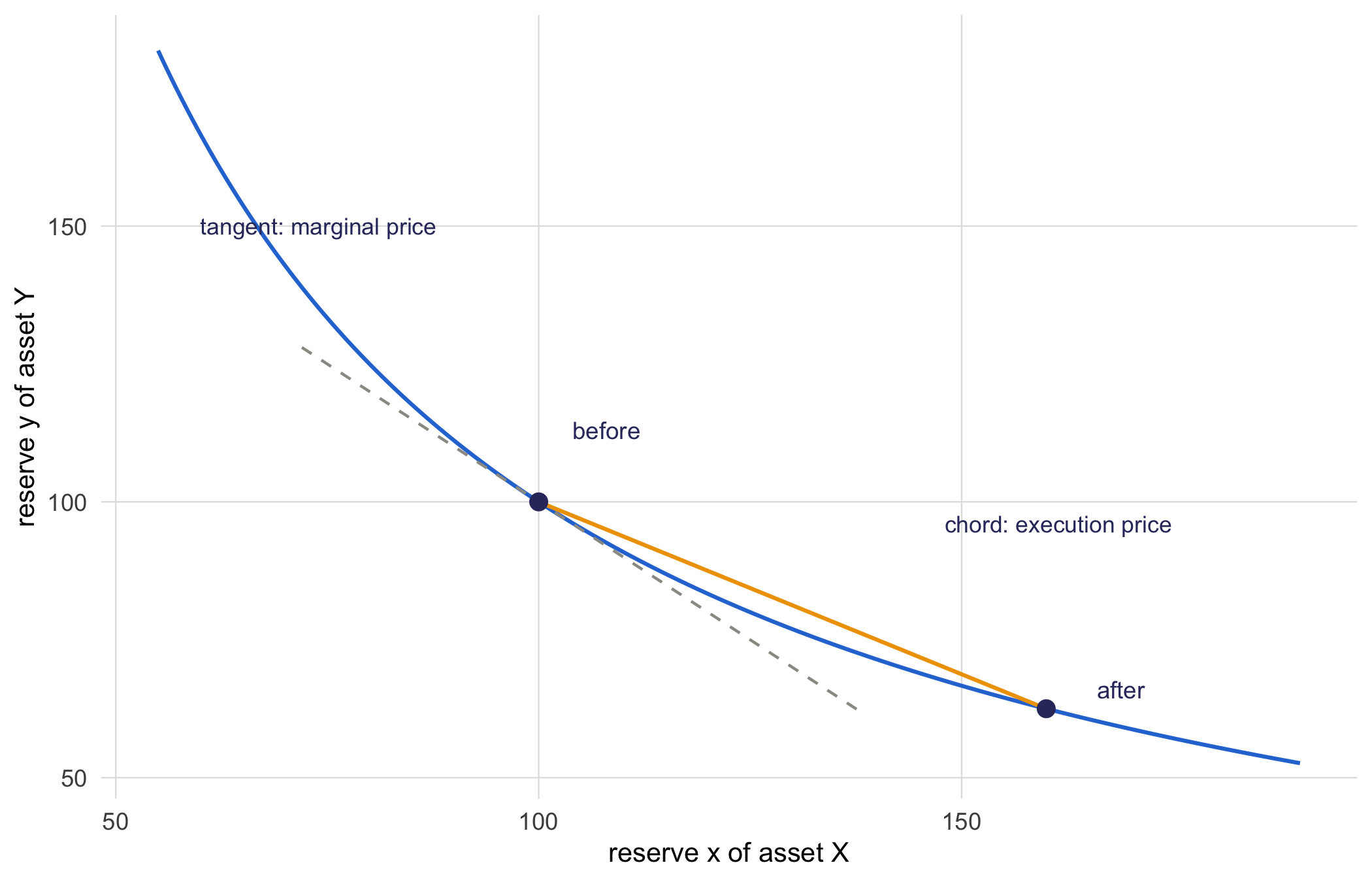
Execution price degrades with trade size. For a finite purchase the trader pays, on average, \(\mathrm{d}x / \mathrm{d}y = (x + \mathrm{d}x)/y\) per unit of \(Y\), which exceeds the spot price \(p\) by \(\mathrm{d}x / y\). The excess is slippage. It arises because the marginal price along the invariant, \(m(x) = x/y = x^2/k\), is convex in the reserve, so that the average price paid while traversing a finite interval sits strictly above the price at the starting point. That is Jensen’s inequality appearing for the first time in this chapter, and it returns below in a more consequential role.

We can pause on a single picture that makes the whole mechanism legible. The invariant is a hyperbola, a trade is a step along it, and the chord and the tangent at the starting point are the two prices we have just distinguished (Figure 8.1).

library(ggplot2)
library(tibble)
PAL <- c('#2a78d6', '#1baf7a', '#eda100', '#008300',
         '#4a3aa7', '#e34948', '#e87ba4', '#eb6834')
book_theme <- ggplot2::theme_minimal(base_size = 11) +
  ggplot2::theme(
    panel.grid.minor = ggplot2::element_blank(),
    panel.grid.major = ggplot2::element_line(
      linewidth = 0.25, colour = 'grey88'),
    axis.title = ggplot2::element_text(size = 10),
    legend.position = 'bottom'
  )

k <- 10000
xr <- seq(55, 190, length.out = 200)
curve_df <- tibble(x = xr, y = k / xr)
x0 <- 100; y0 <- k / x0            # before the trade
x1 <- 160; y1 <- k / x1            # after depositing X
slope_tan <- -k / x0^2             # tangent slope at start
tan_df <- tibble(x = c(72, 138),
                 y = y0 + slope_tan * (c(72, 138) - x0))
pts <- tibble(x = c(x0, x1), y = c(y0, y1))

ggplot(curve_df, aes(x, y)) +
  geom_line(colour = PAL[1], linewidth = 0.7) +
  geom_line(data = tan_df, aes(x, y),
            colour = '#9a9a92', linewidth = 0.5, linetype = 2) +
  annotate('segment', x = x0, y = y0, xend = x1, yend = y1,
           colour = PAL[3], linewidth = 0.7) +
  geom_point(data = pts, aes(x, y),
             colour = '#33356b', size = 2.6) +
  annotate('text', x = 104, y = 113, label = 'before',
           hjust = 0, size = 3.1, colour = '#33356b') +
  annotate('text', x = 166, y = 66, label = 'after',
           hjust = 0, size = 3.1, colour = '#33356b') +
  annotate('text', x = 60, y = 150, label = 'tangent: marginal price',
           hjust = 0, size = 3, colour = '#33356b') +
  annotate('text', x = 148, y = 96, label = 'chord: execution price',
           hjust = 0, size = 3, colour = '#33356b') +
  labs(x = 'reserve x of asset X', y = 'reserve y of asset Y') +
  book_theme

Figure 8.1: The constant product x times y equals k is a hyperbola, and a finite trade steps the pool from the before point to the after point along it; the chord joining the two points is flatter than the tangent at the start, so a finite order receives less of asset Y per unit of X than the marginal rate, which is the slippage.

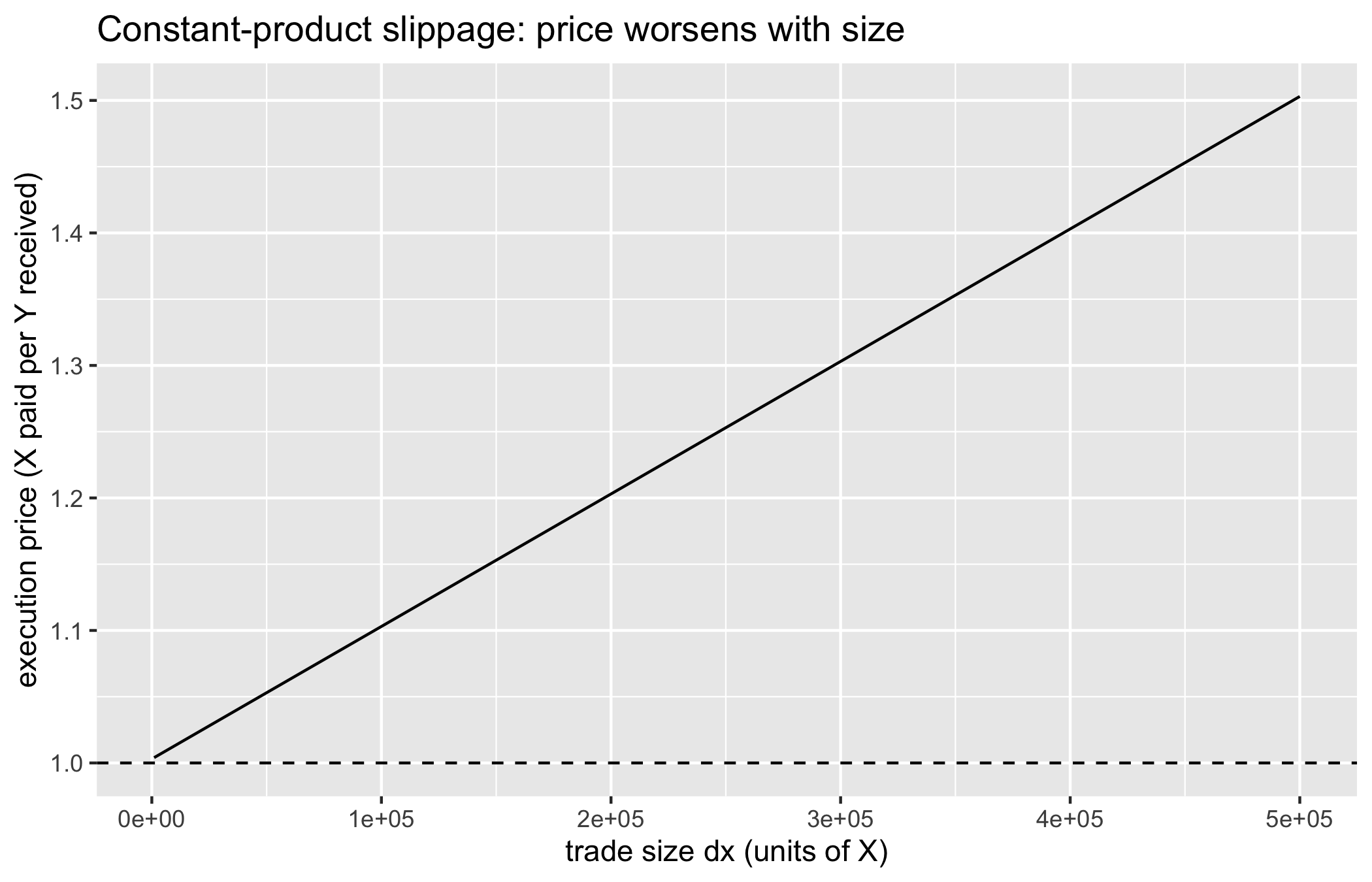
To make the degradation concrete, the verified companion code computes the execution price for a range of trade sizes against a pool that also charges the standard thirty-basis-point fee, and plots the result.

cpmm_out <- function(dx, Rx, Ry, fee = 0.003) {
  dx_eff <- dx * (1 - fee)
  Ry * dx_eff / (Rx + dx_eff)
}

Rx <- 1e6; Ry <- 1e6
sizes <- seq(1e3, 5e5, length.out = 100)
exec_price <- sapply(sizes, function(dx) dx / cpmm_out(dx, Rx, Ry))

ggplot(tibble(size = sizes, price = exec_price), aes(size, price)) +
  geom_line() +
  geom_hline(yintercept = Rx / Ry, linetype = 2) +
  labs(x = 'trade size dx (units of X)',
       y = 'execution price (X paid per Y received)',
       title = 'Constant-product slippage: price worsens with size')

Figure 8.2: Constant-product execution price as a function of trade size. The dashed line is the marginal (spot) price at zero size; a larger order walks further along the hyperbola and pays strictly more.

A trade that consumes a large fraction of the reserves moves the price far, so large orders ‘move the market’ mechanically, with no counterparty required to disagree with them. This is a protocol fact in the sense of Chapter 1: it follows from the invariant by algebra and can be checked by anyone reading the contract.

Check your understanding: slippage of a large order

A CPMM pool holds \(x = 1{,}000{,}000\) units of a stablecoin and \(y = 1{,}000{,}000\) units of a token, so the spot price is one stablecoin per token. Ignoring fees, what average price does a trader pay for a purchase that spends \(\mathrm{d}x = 250{,}000\) stablecoins, and by what fraction does that exceed spot?

The trader receives \(\mathrm{d}y = y\,\mathrm{d}x/(x+\mathrm{d}x) = 10^6 \cdot 2.5\times10^5 / 1.25\times10^6 = 200{,}000\) tokens. The average execution price is \(250{,}000 / 200{,}000 = 1.25\) stablecoins per token, twenty-five percent above the spot price of one. The slippage \(\mathrm{d}x/y = 0.25\) matches the algebra exactly. A quarter of the reserve is a very large order; the point is that the cost is a deterministic function of depth, not a matter of who is on the other side.

8.5 Impermanent loss as a convexity cost

A liquidity provider (LP) deposits both assets into the pool and earns a share of trading fees. The cost of doing so, relative to simply holding the two assets, is impermanent loss (IL). It is the most misunderstood quantity in DeFi, and it is one line of algebra. We dwell on it because it is the hidden term in a pitch a public-health reader will one day be shown: the suggestion that a preparedness fund or an endowment ‘provide liquidity to earn a yield’ on its idle capital. The advertised yield is visible; the convexity cost derived below is not, and a fund treasurer who cannot price it is agreeing to be short volatility without knowing the premium demanded in return.

Suppose the LP deposits when the price of \(Y\) (in units of \(X\)) is \(p_0\), and later the external price has moved to \(p_1\), a gross ratio \(r = p_1 / p_0\). Arbitrageurs keep the pool’s spot price equal to the external price, so at any price \(p\) the reserves satisfy \(x/y = p\) together with \(xy = k\), giving \(x = \sqrt{kp}\) and \(y = \sqrt{k/p}\). The value of the pool position, measured in units of \(X\), is

\[ V_{\text{pool}}(p) \;=\; x + p\,y \;=\; 2\sqrt{k p}. \]

Had the LP instead held the initial reserves \(x_0 = \sqrt{k p_0}\) and \(y_0 = \sqrt{k/p_0}\), the value would be \(V_{\text{hold}}(p_1) = x_0 + p_1 y_0 = \sqrt{k p_0}\,(1 + r)\). Taking the ratio,

\[ \frac{V_{\text{pool}}}{V_{\text{hold}}} \;=\; \frac{2\sqrt{k p_1}}{\sqrt{k p_0}\,(1+r)} \;=\; \frac{2\sqrt{r}}{1 + r}, \]

and the impermanent loss is the shortfall

\[ \mathrm{IL}(r) \;=\; \frac{2\sqrt{r}}{1 + r} - 1 . \]

The interpretation is immediate once we notice what the numerator and denominator are: \(\sqrt{r} = \sqrt{1 \cdot r}\) is the geometric mean of \(\{1, r\}\) and \((1+r)/2\) is their arithmetic mean. Hence

\[ \frac{V_{\text{pool}}}{V_{\text{hold}}} \;=\; \frac{\operatorname{GM}(1, r)}{\operatorname{AM}(1, r)} \;\le\; 1, \]

with equality if and only if \(r = 1\), by the arithmetic-geometric mean inequality, itself a special case of Jensen’s inequality applied to the concave function \(\sqrt{\cdot}\). The pool value is a concave (square-root) function of price while the hold benchmark is linear, and a concave payoff underperforms its own tangent whenever the argument departs from the point of tangency. That is the entire content of impermanent loss.

The mechanism, stated without calculus: the constant-product rule forces the pool to sell the asset that appreciates and buy the asset that depreciates, continuously and in exactly the wrong direction for a trend follower. The LP is structurally short volatility. The companion code gives the closed form and its symmetry.

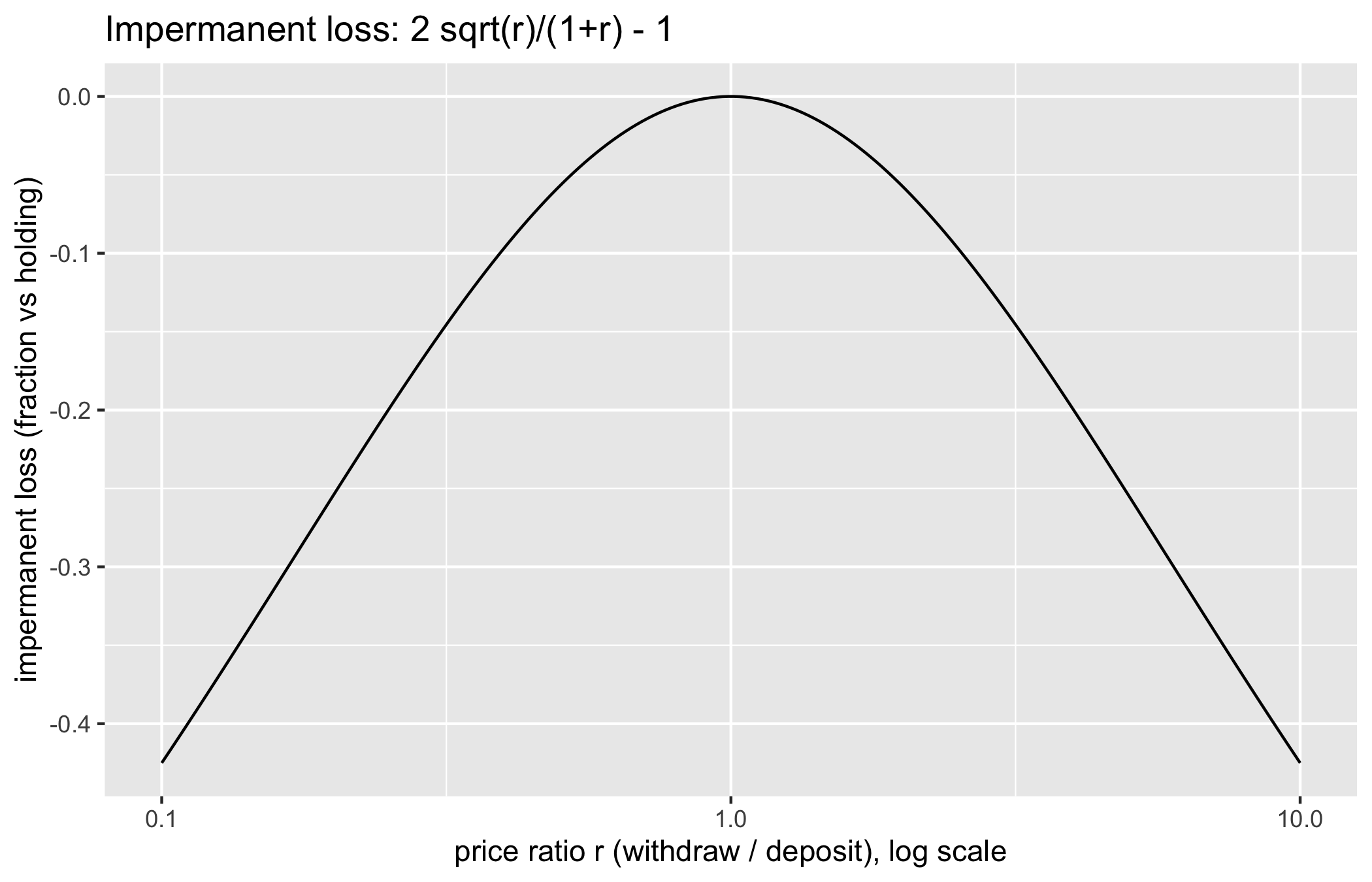
il <- function(r) 2 * sqrt(r) / (1 + r) - 1
r <- 10^seq(-1, 1, length.out = 200)

ggplot(tibble(r = r, il = il(r)), aes(r, il)) +
  geom_line() +
  scale_x_log10() +
  labs(x = 'price ratio r (withdraw / deposit), log scale',
       y = 'impermanent loss (fraction vs holding)',
       title = 'Impermanent loss: 2 sqrt(r)/(1+r) - 1')
c(il_2x = il(2), il_4x = il(4), il_half = il(0.5))
#>       il_2x       il_4x     il_half 
#> -0.05719096 -0.20000000 -0.05719096

Figure 8.3: Impermanent loss against the price ratio r on a log axis. The curve is zero at r = 1, negative on both sides, and symmetric in log r: a doubling and a halving cost the provider the same.

The loss is zero at \(r = 1\), negative on either side, and symmetric in \(\log r\): doubling (\(r = 2\)) and halving (\(r = 1/2\)) cost the same, about two percent, because \(\mathrm{IL}(r) = \mathrm{IL}(1/r)\), a fact the reader can verify directly from the formula. A four-fold move costs about six percent. These are not catastrophic numbers, which is precisely why the loss is survivable when fee income is adequate and ruinous when it is not.

The sceptic’s reflex: ‘impermanent loss is impermanent’

The reassurance that the loss is ‘impermanent’, recovered if the price returns to where it started, is a tier-four narrative presented in the guise of a tier-one fact (Chapter 1). The recovery is conditional on an event, mean reversion, that the provider does not control and cannot assume. What is guaranteed, unconditionally, is the expectation: for any non-degenerate price process the LP realises a negative \(\mathbb{E}[\mathrm{IL}]\) relative to holding, because \(\mathrm{IL}(r) \le 0\) pointwise and equals zero only on a measure-zero set. A more honest name, now common in the literature, is ‘loss versus rebalancing’, or simply the cost of being short gamma. Once it is renamed the matter is clear: the provider is selling volatility and must be paid the premium in fees, or the position is losing.

Check your understanding: why the AM-GM form matters

Someone claims that impermanent loss can be eliminated by choosing a pool whose two assets are ‘highly correlated’, for example two stablecoins. Using the AM-GM characterisation, explain precisely what correlation has to do with it and what it does not change.

Impermanent loss depends only on the realised price ratio \(r = p_1/p_0\) through \(2\sqrt{r}/(1+r) - 1\); it makes no reference to correlation, volatility, or any distributional assumption. What a tightly-correlated pair buys the provider is a distribution of \(r\) concentrated near one, where the curve is flat (its derivative vanishes at \(r = 1\) and the loss is second-order, \(\mathrm{IL} \approx -\tfrac{1}{8}(r-1)^2\) for small moves). So the expected loss is small because \(r\) rarely strays from one, not because the mechanism is different. Correlation shapes the input distribution; the AM-GM inequality still governs the output for every realised value. This is why stablecoin pools are viable LP positions and volatile pairs often are not.

8.6 Lending and liquidation

The second pillar of DeFi is over-collateralised lending, exemplified by Aave and Compound, the two largest decentralised lending protocols. Because borrowers are pseudonymous and cannot be pursued for a deficiency, a loan must be secured by collateral worth more than the debt at all times. A position is described by its collateral value \(C\), its debt \(D\), and a protocol parameter, the liquidation threshold \(\ell \in (0, 1)\). The position is healthy while

\[ \text{health factor} \;=\; \frac{\ell \, C}{D} \;\ge\; 1, \]

and becomes liquidatable the instant the health factor drops below one, at which point liquidators may repay part of the debt in exchange for the borrower’s collateral at a discount. Gudgeon and colleagues analyse the economics of these systems, and the ways in which they fail under stress (Gudgeon, Werner, et al., 2020; Gudgeon, Perez, et al., 2020).

Because collateral value \(C = q \cdot P\) is the quantity of collateral \(q\) times a price \(P\) that the protocol reads from an oracle, the liquidation condition is a threshold on price. Solving \(\ell q P = D\) gives the liquidation price

\[ P^\star \;=\; \frac{D}{\ell \, q}. \]

Below \(P^\star\) the position is under water. The following self-contained illustration computes the health factor and liquidation price for a concrete position.

health_factor <- function(units, price, debt, liq_threshold) {
  liq_threshold * units * price / debt
}

# SYNTHETIC position: 10 units of collateral at a
# current price of 100, a 500-unit stablecoin debt,
# and an Aave-style liquidation threshold of 0.8.
units <- 10; debt <- 500; ell <- 0.8
liq_price <- debt / (ell * units)

c(current_price = 100,
  current_hf = health_factor(units, 100, debt, ell),
  liquidation_price = liq_price)
#>     current_price        current_hf liquidation_price 
#>             100.0               1.6              62.5

The position is healthy at a health factor of 1.6 and is liquidated once the collateral price falls to 62.5, a thirty-seven percent drawdown. The danger is that liquidation is itself a sale: the liquidator sells the seized collateral into the market, which pushes the price down, which drops the next-nearest position below its own threshold. Forced selling begets forced selling. The following compact deterministic model makes the cascade visible: a synthetic population of leveraged positions, an initial price shock, and a fixed price impact per unit liquidated.

simulate_liq_cascade <- function(price0 = 100, shock = -8,
                                 n = 400, leverage = 10,
                                 impact = 0.15) {
  set.seed(7)
  # SYNTHETIC entry prices; longs liquidate at
  # entry * (1 - 1/leverage).
  entry <- rnorm(n, price0, 5)
  liq_price <- entry * (1 - 1 / leverage)
  price <- price0 + shock
  liquidated <- 0L
  repeat {
    newly <- sum(liq_price >= price) - liquidated
    if (newly <= 0) break
    liquidated <- liquidated + newly
    price <- price - impact * newly / n * price0
  }
  list(final_price = price,
       fraction_liquidated = liquidated / n)
}

cascade <- simulate_liq_cascade()
c(final_price = round(cascade$final_price, 2),
  fraction_liquidated = cascade$fraction_liquidated)
#>         final_price fraction_liquidated 
#>             77.0400              0.9975

An eight percent shock is amplified by the feedback loop into a much larger price decline and nearly the entire population of leveraged positions liquidated. The same avalanche structure recurs across this book: a small exogenous disturbance amplified by a structural feedback, as in the mining fork rate of Chapter 5 and the restaking tail of Chapter 10. The statistician’s contribution is to notice that the cascade’s severity is not random but a computable function of the leverage distribution, the threshold, and the depth of the market into which collateral is sold.

8.7 Oracles and flash loans

Every mechanism above consults a price. On a chain that price must come from somewhere, and the somewhere is an oracle: a contract or a signed feed that reports an off-chain quantity to on-chain code. The oracle is the trust boundary of DeFi. Everything upstream of it can be trust-minimised by the consensus machinery of the preceding chapters; the oracle is where an external number, and with it an external assumption, re-enters. A protocol that prices collateral off the current spot price of an on-chain pool has, in effect, delegated its solvency to whoever can move that pool.

Flash loans make that delegation dangerous. A flash loan is an uncollateralised loan of arbitrary size that must be borrowed and repaid within a single transaction; atomicity guarantees that if the repayment fails the entire transaction reverts, so the lender bears no credit risk. This is a genuine and elegant primitive with legitimate uses (arbitrage, collateral swaps, self-liquidation). It is also the ideal instrument for oracle manipulation, because it hands an attacker unlimited capital for the length of one block with no requirement to already possess it. The canonical attack: borrow a large sum, use it to distort a spot-price oracle, transact against a second protocol that trusts that oracle, and unwind, all atomically.

The following self-contained numeric example makes the extraction concrete. A lending market prices a collateral token off the spot price of a single CPMM pool. An attacker flash-borrows stablecoins, buys the collateral token to pump its reported price, and shows how much the naive valuation overstates the true value.

swap_x_for_y <- function(dx, Rx, Ry) {
  dy <- Ry * dx / (Rx + dx)
  list(dy = dy, Rx = Rx + dx, Ry = Ry - dy)
}

# SYNTHETIC pool used naively as a price oracle:
# 1e6 stablecoin (X) and 1e6 collateral token (Y),
# so the honest spot price of the token is 1.
Rx0 <- 1e6; Ry0 <- 1e6
spot0 <- Rx0 / Ry0

loan <- 5e5                       # flash-borrowed stablecoins
after <- swap_x_for_y(loan, Rx0, Ry0)
spot1 <- after$Rx / after$Ry      # manipulated spot price

bought <- after$dy                # collateral acquired
ltv <- 0.75
naive_value <- bought * spot1
true_value <- bought * spot0
borrowable <- naive_value * ltv

c(spot_before = spot0, spot_after = spot1,
  collateral_bought = round(bought),
  naive_valuation = round(naive_value),
  borrowable_at_75pct = round(borrowable),
  true_value = round(true_value),
  bad_debt = round(borrowable - true_value))
#>         spot_before          spot_after   collateral_bought     naive_valuation 
#>                1.00                2.25           333333.00           750000.00 
#> borrowable_at_75pct          true_value            bad_debt 
#>           562500.00           333333.00           229167.00

A single half-million swap more than doubles the reported price. A lending market that valued the acquired collateral at the manipulated spot and lent seventy-five percent against it would advance far more than the collateral is truly worth, leaving bad debt on its books the moment the pool price snaps back after the attacker unwinds. The extraction is deterministic, not probabilistic; it follows from the invariant.

The defence is a matter of estimator design, which is why it is the statistician’s natural territory. A time-weighted average price (TWAP) over \(N\) blocks replaces the single-block spot with a mean; to move a TWAP an attacker must hold the pool displaced for many blocks, paying arbitrage losses each one, which raises the cost of manipulation by roughly a factor of \(N\) and exposes the position to being traded against. Median-of-quorum feeds and signed off-chain prices trade manipulation resistance for a different trust assumption, namely the honesty of the reporters. There is no assumption-free oracle; there is only a choice of which variance and which adversary one prefers. The audit question of the statistician’s second contribution, above, is exactly this: which is it, and what does moving it cost?

The reader will note that nothing in this argument is special to a price. A parametric health instrument that reads a case count from a surveillance feed, an outcome-event tally from the trial ledger, or a breach count from the cold-chain record faces the identical question. A single reporting authority is the equivalent of a single-block spot price, cheap for an interested party to distort; a quorum of independent surveillance sources, or a multi-day average of reported cases, is the equivalent of a TWAP, more costly to move but slower to respond. This is precisely the tension the World Bank’s bonds resolved, in the event, on the side of slowness. The conservative multi-condition trigger was a manipulation-resistant estimator purchased at the price of a delayed and partial payout, and whether that was the right trade is a question of estimator design, not of blockchain engineering.

8.8 Stablecoins

A stablecoin is a token engineered to hold a constant value, almost always one United States dollar. Moin and colleagues, in their systematisation of the subject (Moin et al., 2020), classify the designs by what backs the peg, and the taxonomy is worth committing to memory because the failure modes follow from it.

Fiat-collateralised. Each token is a claim on a dollar held by a custodian (Tether, USDC). The peg is only as good as the custodian’s reserves and redemption policy; this is a tier-two empirical claim about a balance sheet, auditable in principle, and reintroduces exactly the trusted intermediary the chain claimed to remove.
Crypto-collateralised. Each token is backed by an over-collateralised position in volatile crypto assets (Dai). Solvency is maintained by the same liquidation machinery as a lending market, and it inherits the same cascade risk when the collateral falls fast.
Algorithmic. The peg is defended not by collateral but by a control rule that expands and contracts supply, often coupled to a companion ‘governance’ or ‘seigniorage’ token. This is the fragile design, and the fragility is analysable.

We collect the taxonomy in one place, since the failure mode of each design follows directly from what backs the peg (Table 8.2).

Table 8.2: Stablecoin designs classified by what backs the peg, with the peg mechanism, the characteristic failure mode, and a canonical example of each

Collateral class	Peg mechanism	Failure mode	Example
Fiat-reserve	Redeemable one-for-one against custodial dollars	Reserve shortfall or a frozen redemption window	USDC
Crypto over-collateralised	Over-collateralised vault defended by liquidation	Collateral crash outruns the liquidators	DAI
Algorithmic	Mint-and-burn against a companion token	Reflexive depeg spiral	TerraUSD

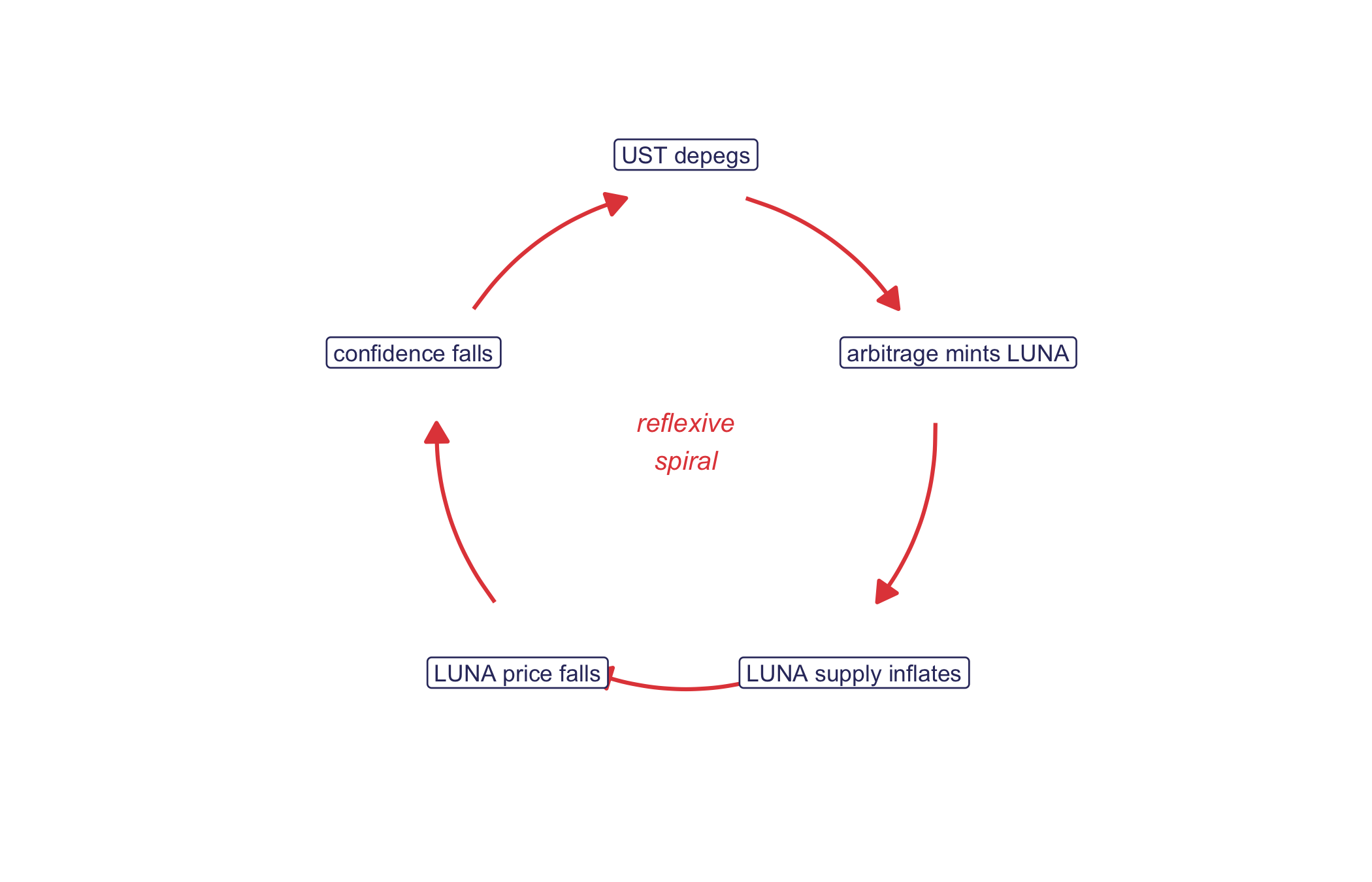
Algorithmic stablecoins are reflexive: the mechanism that defends the peg depends on the price of a second token whose value depends, in turn, on confidence in the peg. Klages-Mundt and Minca (Klages-Mundt & Minca, 2019) show how such systems admit multiple equilibria, a stable peg and a collapse, with no restoring force between them once confidence breaks. The canonical realisation was the collapse of TerraUSD (UST) and its companion token Luna in May 2022, which Briola and colleagues (Briola et al., 2023) anatomise in detail. UST maintained its peg by a mint-and-burn arbitrage: one UST was always redeemable for one dollar of newly minted Luna. When UST slipped below the peg under redemption pressure, defending it minted ever more Luna, whose price collapsed under the new supply, which destroyed the very backing the arbitrage relied on, which in turn accelerated the redemptions. The feedback loop is the same positive-feedback deleveraging spiral as the liquidation cascade above, differing only in that here the forced selling is of the collateral asset the protocol itself creates. Tens of billions of dollars of notional value evaporated in days.

The mechanism is easiest to see as a loop, in which each step feeds the next and the whole turns faster the further the peg slips (Figure 8.4).

ang <- 90 - (0:4) * 72
rad <- ang * pi / 180
nodes <- tibble(
  x = cos(rad), y = sin(rad),
  lab = c('UST depegs', 'arbitrage mints LUNA',
          'LUNA supply inflates', 'LUNA price falls',
          'confidence falls')
)
nx <- nodes$x; ny <- nodes$y
bx <- nodes$x[c(2:5, 1)]; by <- nodes$y[c(2:5, 1)]
t <- 0.22                          # trim arrows clear of boxes
edges <- tibble(
  x = nx + t * (bx - nx), y = ny + t * (by - ny),
  xend = nx + (1 - t) * (bx - nx), yend = ny + (1 - t) * (by - ny)
)

ggplot() +
  geom_curve(data = edges,
             aes(x = x, y = y, xend = xend, yend = yend),
             curvature = -0.18, colour = '#e34948', linewidth = 0.7,
             arrow = grid::arrow(length = grid::unit(0.28, 'cm'),
                                 type = 'closed')) +
  geom_label(data = nodes, aes(x, y, label = lab),
             colour = '#33356b', fill = 'white',
             linewidth = 0.3, size = 3,
             label.r = grid::unit(0.15, 'lines')) +
  annotate('text', x = 0, y = 0, label = 'reflexive\nspiral',
           colour = '#e34948', size = 3.4, fontface = 'italic') +
  coord_equal(clip = 'off') +
  xlim(-1.6, 1.6) + ylim(-1.4, 1.4) +
  theme_void()

Figure 8.4: The TerraUSD collapse as a reflexive loop: a depeg triggers arbitrage that mints the companion token LUNA, whose inflating supply drives its price down, which erodes the confidence backing the peg and deepens the depeg, so the loop accelerates the very collapse it was meant to arrest.

The epidemiologist will recognise the shape of this dynamic. A reflexive collapse is a positive-feedback process, and it is tempting to read the UST spiral as the financial cousin of a panic-driven demand spike in an outbreak, in which fear of shortage provokes hoarding, which produces the very shortage that was feared, which deepens the fear. The formal resemblance is genuine: in both cases a quantity that measures confidence, the token price or the perceived availability of a commodity, feeds back on the behaviour that determines it, and both admit a stable branch and a runaway branch separated by a threshold. We should, however, be candid about where the analogy ends. An epidemic spike is driven by human belief and can be arrested by reassurance, by resupply, or by information, because the feedback runs through people who can be addressed; the UST spiral was, once past its threshold, a mechanical arbitrage executed by code against a supply schedule, with no reassurance available to a smart contract and no authority positioned to inject restoring capital in time. The analogy is useful for intuition about the existence of tipping points; it is misleading if it suggests that the interventions which calm a human panic would have saved an algorithmic peg. Broadening the view, Werner and colleagues, in a systematisation of the field (Werner et al., 2022), place these mechanisms, their oracles, and their attack surfaces in a single framework worth reading in full.

The sceptic’s reflex: a high APY is usually emission

An advertised yield of, say, eighty percent annually is a tier-four narrative until decomposed. Write it as \(\text{APY} = \text{fees} + \text{emission}\). The fee component is real income: counterparties paid it for a service. The emission component is freshly minted governance tokens handed to liquidity providers, funded by dilution of existing holders, and it evaporates when the emission schedule tapers or the token price falls, which are correlated events. A yield that is predominantly emission is a wealth transfer from later to earlier participants, structurally identical to the token-unlock overhang studied in Chapter 11. Before believing a yield, ask for its two components separately. Protocols that cannot or will not provide the split are answering the question by refusing it.

The decomposition generalises past the two-way fee-versus-emission split. A headline yield is a sum over sources, and only some of them are income a counterparty actually paid (Table 8.3).

Table 8.3: The four sources of an advertised yield, of which only the first two are income a counterparty paid; the last two are transfers that decay or reverse

Source	Real cash flow?	Sustainable?	Test
Trading fees	Yes	Yes, while volume persists	Trace it to observed pool volume
Lending interest	Yes	Yes, while borrowers pay	Trace it to borrower demand
Token emission	No	No, decays as the schedule tapers	Read the emission schedule
New-entrant capital	No	No, a transfer not an earning	Ask who is paying whom

8.8.1 Public-health connection: parametric escrow

We now return to the instrument with which the chapter opened and assemble it from the parts we have derived. A smart contract that pays out automatically on a verifiable trigger is the escrow of parametric insurance, in which the payout is tied not to an assessed loss but to an objective index: rainfall below a threshold, a wind speed above a cutoff, or an epidemic case count crossing a level. The conditional-escrow contract holds the premium capital and releases it the instant the index, delivered by an oracle, crosses the trigger. For public-health financing the intuitive appeal is real: a preparedness fund could disburse to a ministry of health the day a notifiable-disease surveillance feed crosses an outbreak threshold, with no claims adjudication and no discretionary delay, and the escrow’s solvency and payout logic would be auditable by anyone. This is, in outline, what the World Bank’s 2017 bonds attempted.

The candour we owe the pitch is this: the contract does not solve the hard problem, it relocates it. Everything reduces to the trigger and the oracle that reports it. Did the outbreak truly occur at the reported scale? Was the surveillance feed accurate, timely, and free of manipulation by a party with a financial stake in the outcome? Was the threshold set low enough to fire when help was needed, and high enough not to fire spuriously? These are the same questions, and the same trust boundary, as the price oracle of the previous section, and a blockchain answers none of them. The mathematics of the escrow is trivial; the epidemiology and the data integrity of the trigger are the entire problem, and they live off-chain.

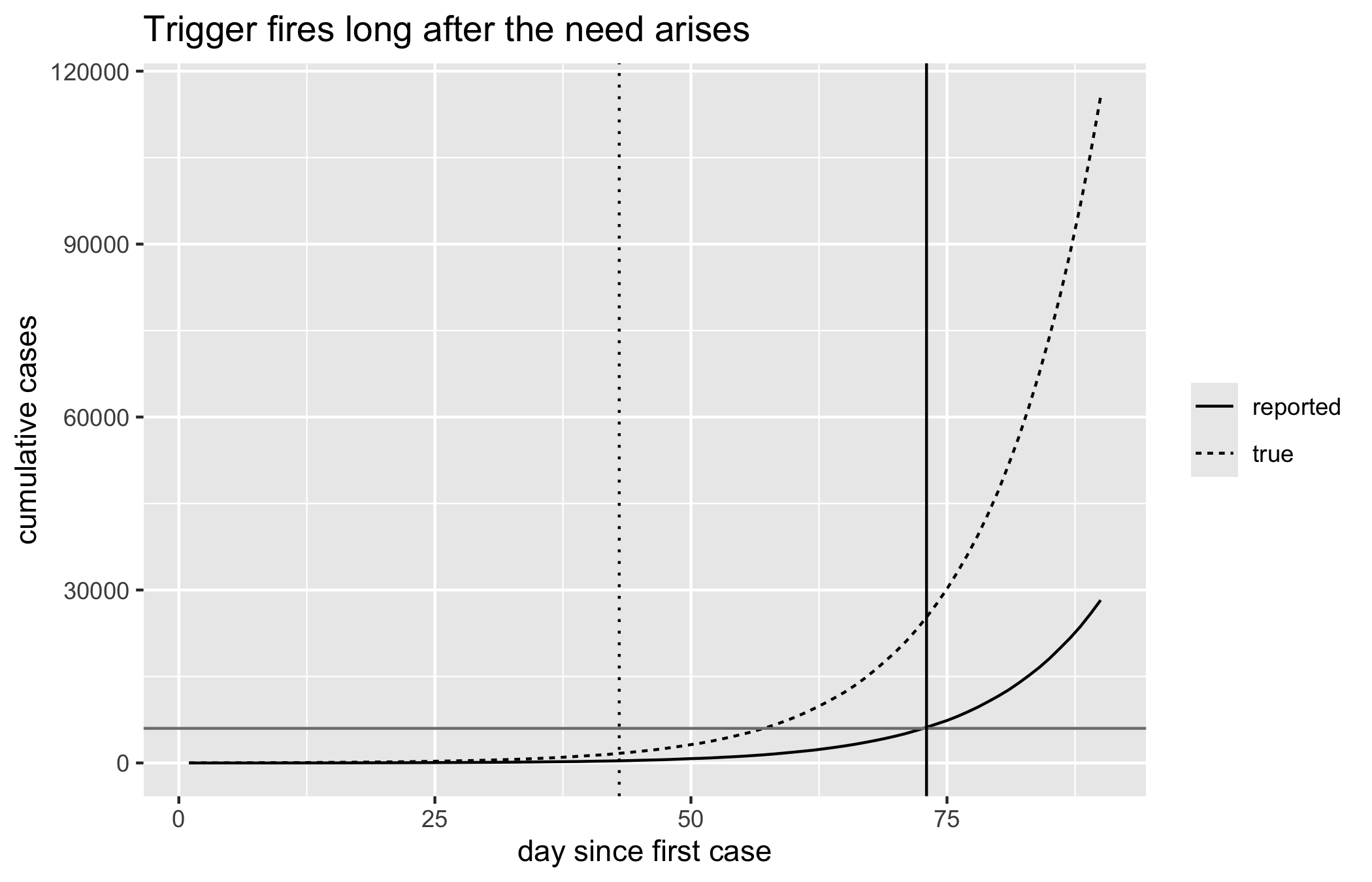
To see how the trigger, rather than the plumbing, governs the outcome, consider a stylised outbreak. To illustrate, suppose a preparedness bond promises a fixed disbursement, and its trigger requires the reported cumulative case count to exceed a fixed threshold. The epidemic itself grows roughly exponentially in its early phase, but the reporting is neither instantaneous nor complete: cases are observed with a delay and a detection probability below one, so the count the oracle sees lags the count that exists. A conservatively high threshold, chosen to avoid paying out on a false alarm, then fires only well after the true burden has mounted. The following synthetic computation traces the true and reported curves and marks the day the trigger fires against the day the funds were first needed.

set.seed(7)
days <- 1:90
# SYNTHETIC early-epidemic incidence: roughly
# exponential growth with Poisson noise.
growth <- 0.09
new_true <- rpois(length(days), lambda = 3 * exp(growth * days))

# Reporting: a detection probability below one and a
# fixed reporting delay in days.
detect <- 0.6
delay <- 10
detected <- rbinom(length(days), size = new_true, prob = detect)
reported_by_day <- numeric(length(days))
for (i in seq_along(days)) {
  j <- i + delay
  if (j <= length(days)) reported_by_day[j] <- detected[i]
}

cum_true <- cumsum(new_true)
cum_reported <- cumsum(reported_by_day)

# 'Need' level: true burden at which the response
# should begin. Conservative payout threshold: set on
# the REPORTED count to avoid a false alarm.
need_level <- 1500
threshold <- 6000
need_day <- days[which(cum_true >= need_level)[1]]
trigger_day <- days[which(cum_reported >= threshold)[1]]

curves <- tibble(day = days, true = cum_true,
                 reported = cum_reported) |>
  pivot_longer(c(true, reported),
               names_to = 'series', values_to = 'cases')

ggplot(curves, aes(day, cases, linetype = series)) +
  geom_line() +
  geom_hline(yintercept = threshold, colour = 'grey50') +
  geom_vline(xintercept = need_day, linetype = 3) +
  geom_vline(xintercept = trigger_day) +
  labs(x = 'day since first case', y = 'cumulative cases',
       linetype = NULL,
       title = 'Trigger fires long after the need arises')

c(need_day = need_day, trigger_day = trigger_day,
  lag_days = trigger_day - need_day,
  true_burden_at_trigger = cum_true[trigger_day])
#>               need_day            trigger_day               lag_days 
#>                     43                     73                     30 
#> true_burden_at_trigger 
#>                  25273

Figure 8.5: SYNTHETIC outbreak. The true cumulative case curve (solid) rises ahead of the reported curve (dashed), because reporting is delayed and incomplete. A conservatively high payout threshold (horizontal line) is crossed by the reported curve only on the trigger day (solid vertical line), long after the day the response was first needed (dotted vertical line).

The delay is not a defect of the escrow, which would pay the instant it was commanded; it is a property of the trigger and its feed. The reported curve lags the true curve by the reporting delay and sits below it by the detection shortfall, so that a threshold set conservatively high, in order not to disburse on a false alarm, is crossed only after the true burden has climbed to many times the level at which help was first warranted. On the one hand a lower threshold would fire sooner, and on the other it would fire on noise and on outbreaks that fizzle, disbursing scarce capital when no response was needed. That trade-off, between the sensitivity and the specificity of the trigger, is the whole design problem, and it is the epidemiologist’s problem, not the programmer’s. This is the lesson of the World Bank’s experience, reproduced here in miniature.

Most ‘DeFi for health financing’ pitches fail the test

The recurring proposal to fund health programmes through DeFi yields conflates two things a statistician should keep apart. The escrow-and- trigger logic is sound and modest, and where a donor and a recipient lack a common trusted intermediary, an auditable conditional payout has real value. The yield-generation layer, staking the premium float in a lending market or a liquidity pool to ‘grow the fund’, imports impermanent loss, liquidation cascades, oracle-manipulation risk, and smart-contract risk onto capital that is supposed to be there when an outbreak hits, which is exactly when those risks correlate and fire together. A preparedness fund is not the place to be short gamma. As Chapter 1 warns, if a trusted custodian already exists or can be appointed, a well-governed account with an audit log delivers the auditable payout without the tail risk. Adopt the escrow logic; refuse the yield farming.

8.9 Worked example: decomposing a liquidity provider’s return

The chapter’s threads converge on the practical question a would-be liquidity provider, and equally the treasurer of a fund tempted to ‘earn a yield on the float’, must answer: does the fee income outrun the impermanent loss? The net return over a period, relative to holding, is

\[ \text{net} \;=\; \underbrace{f \cdot \tfrac{t}{365}}_{\text{fee yield}} \;-\; \underbrace{\bigl(-\mathrm{IL}(r)\bigr)}_{\text{IL cost}}, \]

where \(f\) is the annualised fee yield the position earns from trading volume, \(t\) is the holding period in days, and \(r\) is the realised price ratio. The following computes the decomposition across a grid of price moves and two fee environments.

scenarios <- expand_grid(
  price_move = c(1.00, 1.25, 1.50, 2.00),
  fee_apr = c(0.05, 0.20)
) |>
  mutate(
    r = price_move,
    il_cost = -il(r),                 # positive = loss vs hold
    fee_yield = fee_apr * 30 / 365,   # 30-day holding period
    net = fee_yield - il_cost
  )

scenarios |>
  select(price_move, fee_apr, il_cost, fee_yield, net)
#> # A tibble: 8 × 5
#>   price_move fee_apr il_cost fee_yield      net
#>        <dbl>   <dbl>   <dbl>     <dbl>    <dbl>
#> 1       1       0.05 0         0.00411  0.00411
#> 2       1       0.2  0         0.0164   0.0164 
#> 3       1.25    0.05 0.00619   0.00411 -0.00208
#> 4       1.25    0.2  0.00619   0.0164   0.0102 
#> 5       1.5     0.05 0.0202    0.00411 -0.0161 
#> 6       1.5     0.2  0.0202    0.0164  -0.00377
#> 7       2       0.05 0.0572    0.00411 -0.0531 
#> 8       2       0.2  0.0572    0.0164  -0.0408

Read the table as the LP’s decision problem. When the price barely moves (\(r = 1\)) impermanent loss is zero and every basis point of fee is profit. As the price move grows the IL cost rises quadratically at first and overwhelms a thin fee yield: at a five-percent fee environment a fifty-percent price move already leaves the provider behind a simple hold, whereas the same move is survived comfortably when fees run at twenty percent. The break-even is the locus where the two columns cancel, and it is the only number that matters for the decision. Notice what is absent: any governance-token emission. Had the protocol advertised its yield inclusive of emission, the fee_yield column would be inflated by a component that is dilution rather than income, and the break-even analysis would be correspondingly optimistic. Decomposing the yield before running this table is the discipline the chapter has been arguing for throughout.

8.10 Collaborating with an LLM

A language model is a capable assistant for DeFi mathematics and a dangerous one for DeFi claims. It may be used to derive and to draft, but the economics should be verified independently.

Prompt: ‘Derive the impermanent loss of a constant-product pool as a function of the price ratio and show it is symmetric in log price.’ Watch for: sign errors, a missing factor of two, or a confident derivation that silently assumes zero fees or a fifty-fifty pool without saying so. Verification: check the closed form against il(2) and il(0.5) in the code above; if the model’s formula disagrees at \(r = 2\), it is wrong, and the one-line evaluation settles it.
Prompt: ‘Explain how a flash loan can manipulate this lending protocol’s oracle and estimate the extractable value.’ Watch for: a fluent narrative that omits the atomic-repayment constraint, ignores the fee and slippage the attacker pays to move the pool, or fails to note that a TWAP oracle would defeat the attack. Verification: reproduce the extraction as a small numeric example, as in the oracle chunk, and confirm the attacker’s round-trip actually nets positive after its own slippage.
Prompt: ‘This protocol advertises a 120-percent APY. Is it sustainable?’ Watch for: the model taking the headline at face value or inventing a reserves figure. Verification: insist on the fee-versus-emission decomposition; a sustainable yield is a real cash flow from counterparties, and if the model cannot source the fee component from actual volume, treat the number as emission until shown otherwise.

8.11 Exercises

Slippage bound. For a no-fee constant-product pool with reserves \((x, y)\), prove that the average execution price of a purchase of size \(\mathrm{d}x\) is exactly \((x + \mathrm{d}x)/y\), and hence that fractional slippage relative to spot equals \(\mathrm{d}x/x\). Confirm numerically against cpmm_out() with the fee set to zero.
Impermanent loss is second order. Show by Taylor expansion that \(\mathrm{IL}(r) \approx -\tfrac{1}{8}(r - 1)^2\) near \(r = 1\), and hence that for small price moves the loss scales with the square of the move. Verify the approximation against il() for \(r \in \{1.01, 1.05, 1.1\}\) and report the relative error.
Break-even fee yield. Using the LP decomposition, derive the annualised fee yield \(f\) that exactly offsets the impermanent loss of a given realised price ratio \(r\) over a 30-day period. Tabulate the break-even \(f\) for \(r \in \{1.25, 1.5, 2, 4\}\) and comment on which pools are viable LP positions.
Liquidation price and cascade sensitivity. Extend simulate_liq_cascade() to sweep the leverage parameter over \(\{2, 5, 10, 20\}\) and plot the fraction liquidated against leverage for a fixed initial shock. Explain the shape in terms of the liquidation-price formula \(P^\star = D/(\ell q)\).
Oracle manipulation cost. Modify the flash- loan example so the lending market prices collateral off a TWAP over \(N\) blocks rather than the single-block spot. Argue, and illustrate numerically, why the attacker’s cost to move the reported price scales with \(N\), and state the assumption about inter-block arbitrage that the argument requires.
Reflexivity of an algorithmic peg. Write a minimal two-state model of a mint-and-burn stablecoin in which the backing token’s price is a decreasing function of its supply. Identify the two equilibria of Klages-Mundt & Minca (2019) and the confidence threshold that separates them, and relate the collapse branch to the TerraUSD account of Briola et al. (2023).
Parametric trigger sensitivity and specificity. Using the synthetic outbreak of Figure 8.5, sweep the payout threshold over a range of values and, for each, record the lag between the need day and the trigger day. Then introduce a second, non-epidemic scenario in which reported cases plateau below the true outbreak level, and report for each threshold whether the trigger fires spuriously. Explain the sensitivity-specificity trade-off this exposes, and argue why it, and not the escrow contract, is the binding constraint on a parametric health bond.

8.12 Further reading

The Uniswap v2 (Adams et al., 2020) and v3 (Adams et al., 2021) specifications are the primary sources for the constant-product and concentrated-liquidity market makers; read v2 first, since its invariant is the one derived here and v3 is a change of variables on the same idea. The mathematical theory of constant-function markets, including when prices are well-defined and how curvature governs slippage and loss, is developed rigorously by Angeris & Chitra (2020) and Angeris et al. (2021); these are the papers that turn AMMs from an engineering trick into an object with theorems. For lending and its instabilities, Gudgeon, Werner, et al. (2020) models the interest-rate mechanisms and Gudgeon, Perez, et al. (2020) analyses how they behave under stress. The stablecoin landscape is mapped by the systematisation of Moin et al. (2020), and the specific instability of algorithmic designs by Klages-Mundt & Minca (2019), with the TerraUSD collapse dissected empirically by Briola et al. (2023). Finally, the DeFi systematisation of Werner et al. (2022) is the single best map of the whole territory, oracles, flash loans, composability risk, and the attack surface they jointly create, and it is the reference to keep at hand when reading any new protocol.

8.13 In conclusion

In conclusion, three points are to be emphasized. First, the mechanisms of decentralised finance, once stripped of their promotional language, are elementary and auditable: a swap is a move along a level set, impermanent loss is the arithmetic- geometric mean inequality made financial, a liquidation is a threshold crossing, and each admits a closed form a statistician can check in a line. Second, in every one of these mechanisms the oracle is the assumption that matters, and the public-health instrument that motivated the chapter inherits exactly this: a parametric bond is only as sound as the surveillance feed that reports its trigger, and the choice between a fast, manipulable index and a slow, robust one is a problem of estimator design, as the World Bank’s experience with its 2017 pandemic bonds makes plain. Third, the escrow-and-trigger logic merits adoption where no common trusted custodian exists, but the yield-generation layer that is so often bolted onto it, and which imports impermanent loss, liquidation cascades, and oracle risk onto capital that must be present precisely when those risks fire together, should be refused, since a preparedness fund is not the place to be short gamma, and where a well-governed account with an audit log will serve, it is to be preferred.